Shelf life
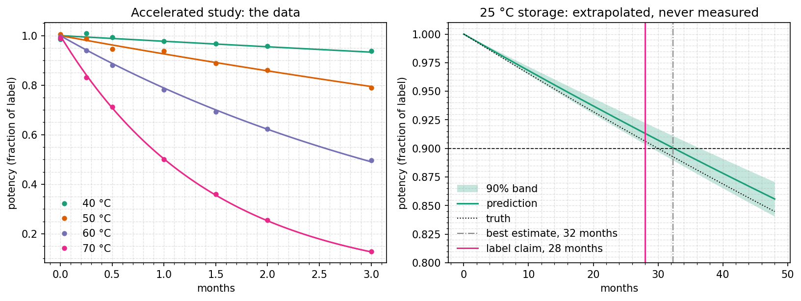
How long does a drug keep its potency? At the storage temperature it degrades too slowly to measure in a few months, so an accelerated study stores it hot, measures for three months, and extrapolates the rate down to 25 °C. The answer that goes on the label is not the best estimate. It is the one-sided 95% lower bound on the shelf life, so this example's result is a statement about uncertainty, and the uncertainty decides it.
It needs no sampler: the maximum likelihood, the Fisher information and a profile likelihood are enough. Read the uncertainty guide for the methods themselves.
Run it
uv run python examples/shelf_life/shelf_life.py
uv run python examples/shelf_life/shelf_life.py --no-plot
About 20 seconds on CPU. Prints the fit, the rate's uncertainty at each temperature and the shelf life, and writes shelf_life.png to examples/shelf_life/figures/.
XLA may print Algebraic simplifier is likely stuck to stderr while this compiles. It is harmless; see Troubleshooting.
The model
Potency
The study stores the drug at 40, 50, 60 and 70 °C and assays it 7 times over three months, with a 1% assay standard deviation. The data are drawn from a known truth: 90% potency after 30 months at 25 °C, and
The law is written around 25 °C because
The initial potency is fixed at
def rate(log_k25: Any, ea_over_r: Any, temperature_c: Any) -> Any:
    """Arrhenius, written around 25 °C so ``log_k25`` is the rate the label needs."""
    return jnp.exp(log_k25 - ea_over_r * (1 / (273.15 + temperature_c) - 1 / STORAGE_K))


def simulate_fn(predictors: Any, ts: Any, covariates: Any, y0: Any, solver: Any) -> Any:
    k = rate(
        predictors["log_k25"].value, predictors["Ea_over_R"].value, covariates["temperature_C"]
    )
    return solver.diffeqsolve(diffrax.ODETerm(lambda t, y, args: -k * y), ts, y0)


model = hm.HybridModel(
    predictors={
        "log_k25": hm.Parameter(-4.0, bounds=(-12.0, 0.0)),
        "Ea_over_R": hm.Parameter(10000.0, bounds=(2000.0, 30000.0)),
    },
    simulate_fn=simulate_fn,
    state_to_output=lambda state: state,
    output_channel_names=("potency",),
    solver=hm.SolverConfig(rtol=1e-8, atol=1e-10),
)
The fit and its information
The trainer gets close, and optimize finishes at the maximum likelihood. noise_sd="data" uses the assay variance given with each measurement, and log_prior=None keeps this a likelihood-only problem:
fit = model.fit(
    study, hm.OptaxTrainingConfig(steps=1500, lr=0.05), key=jr.key(1), verbose=False
)
problem = hm.inference.make_problem(fit.model, study, log_prior=None, noise_sd="data")
mle = problem.optimize().problem
fisher = mle.fisher()
print(fisher.summary())Fisher information
estimate std error 95% interval
Ea_over_R 1.217e+04 173.6 [1.183e+04, 1.251e+04]
log_k25 -5.726 0.06914 [-5.862, -5.591]
Strongest correlations
Ea_over_R and log_k25: -0.989
Condition number 174Extrapolating
The rate at any temperature is a line in derived gives the standard error of any function of the values by the delta method, using their covariance, correlation included. Here it is applied to
# log k(T) depends on both values, so its standard error uses their covariance,
# correlation included. derived() takes the gradient and applies it.
print("\nRelative uncertainty of the rate, one standard error:")
spreads = {}
for temperature in (STORAGE_C, *TEST_TEMPERATURES_C):
    log_k = fisher.derived(
        lambda values, t=temperature: jnp.log(rate(values["log_k25"], values["Ea_over_R"], t))
    )
    spreads[temperature] = float(log_k.standard_error)
    note = "  (storage, no data)" if temperature == STORAGE_C else ""
print(f" {temperature:4.0f} °C ±{100 * spreads[temperature]:.1f}%{note}")Relative uncertainty of the rate, one standard error:
25 °C ±6.9% (storage, no data)
40 °C ±4.2%
50 °C ±2.6%
60 °C ±1.3%
70 °C ±1.3%At 25 °C, where nothing was measured, the rate is five times less certain than at 60 or 70 °C. That uncertainty passes straight into the shelf life, which is inversely proportional to
The shelf life
A two-sided 90% interval has a one-sided 95% bound at each end. The fastest plausible rate gives the shortest plausible shelf life, and the claim is that bound rounded down to whole months. The profile likelihood gives the bound without assuming the estimate is Gaussian:
# A two-sided 90% interval has a one-sided 95% bound at each end. The fastest
# plausible rate gives the shortest plausible shelf life.
profile = mle.profile("log_k25", confidence=0.90)
slowest, fastest = profile.interval
if slowest is None or fastest is None:
    raise SystemExit(
        f"the data do not bound the rate, so no claim can be set: {profile.stop_reasons}"
    )
estimate = shelf_life(math.exp(float(mle.physical(mle.position)["log_k25"])))
lower = shelf_life(math.exp(fastest))
label = math.floor(lower)
print(f"\nShelf life at 25 °C: {estimate:.1f} months, best estimate")
print(f" one-sided 95% lower bound {lower:.1f} months, so a label claim of {label} months")Shelf life at 25 °C: 32.3 months, best estimate
one-sided 95% lower bound 28.9 months, so a label claim of 28 monthsThe true shelf life is 30.0 months. A label set from the best estimate would have claimed 32, and the product would have been out of specification for its last two months. The lower bound claims 28.
The delta method gives a bound on any function of the values, with no need to reparametrise. interval(side="lower") makes it one-sided:
# The delta method gives the same kind of bound for any function of the values,
# in one line, but assumes the shelf life itself is close to Gaussian.
life = fisher.derived(lambda values: shelf_life(jnp.exp(values["log_k25"])))
wald, _ = life.interval(confidence=0.95, side="lower")
print(f"  delta method: {float(life.estimate):.1f} ± {float(life.standard_error):.1f} months,")
print(f" one-sided 95% lower bound {float(wald):.1f} months") delta method: 32.3 ± 2.2 months,
one-sided 95% lower bound 28.6 monthsIt is 0.3 months lower than the profile's bound, because it treats the shelf life, which is
At another storage temperature
To claim a shelf life at 30 °C, profile the rate at 30 °C. Write the law around that temperature, so that its rate is a parameter:
def rate(log_k30, ea_over_r, temperature_c):
    return jnp.exp(log_k30 - ea_over_r * (1 / (273.15 + temperature_c) - 1 / 303.15))
The data and the fit are unchanged, since this is the same law with different parameters. Then use mle.profile("log_k30", confidence=0.90) as above. For a quick check without refitting, use derived on the existing fit with rate(values["log_k25"], values["Ea_over_R"], 30.0).
Draws from the estimate's sampling distribution carry its uncertainty into any function of it. FisherResult.sample gives them, and predict turns them into a potency band at 25 °C, a condition the study never ran:
# Draws from the estimate's sampling distribution carry its uncertainty into
# any function of it: here the shelf life, and the potency curve at 25 °C.
draws = fisher.sample(key=jr.key(2), n_draws=4000)
sampled = shelf_life(np.exp(np.asarray(mle.physical(draws)["log_k25"])))
storage = hm.make_experiment(
    channels={"potency": hm.ChannelObs(ts=jnp.asarray([0.0]), values=jnp.asarray([1.0]))},
    covariates={"temperature_C": STORAGE_C},
    y0=[1.0],
    exp_id="25 C",
)
months = jnp.linspace(0.0, 48.0, 97)
band = mle.predict(
    draws, [storage], ts=months, n_draws=400, quantiles=(0.05, 0.95), key=jr.key(3)
)["25 C"]
The draws' 5th percentile of the shelf life is 28.9 months, the same as the profile's bound, because this likelihood is close to Gaussian in
What the interval does not cover
The interval assumes the model. If the degradation is not first order, or Arrhenius does not hold from 70 °C down to 25 °C, for instance because the mechanism changes, the interval says nothing about it. This is why real labels rest on long-term data at the storage condition, evaluated with the same kind of lower bound (ICH Q1E), and why accelerated studies like this one are used to predict them early.
The band is for the mean potency curve. A single assay scatters around it by the assay's 1%.