Custom training loop
The stock trainers — train_with_optax, train_with_evosax — are assembled from public pieces in jaxhybridmodels.training.kernels. If you want a loop the stock trainers do not express — a bespoke schedule, per-bucket weighting, a custom regulariser, a different accumulation rule — you compose those same kernels yourself instead of forking a trainer.
This example recovers a harmonic oscillator's frequency omega from noisy position data using a hand-written loop built from:
build_bucket_step— the jitted per-bucket(loss, grads)kernel (one trace per bucket shape);build_penalty_step— charges a regulariser once per step, outside the bucket loop. Here it is a custom L2 regulariser on one leaf, not the default bound-saturation penalty;build_apply_update— the single optimiser update per step.
It also injects a custom masked-Huber loss and a per-bucket weight at the call sites, exactly where a stock trainer would not let you.
uv run python examples/custom_loop/train_custom_loop.pyThe loop body is the library's definition of a step — one full pass over every bucket, accumulate gradients, then one update. Change the accumulation rule and you have a genuinely different trainer.
The script, in full
The example is a single file with no hidden parts — what you see is what runs:
"""Write your own training loop against the public gradient kernels.

The stock trainer (:func:`jaxhybridmodels.train_with_optax`) is assembled from
public pieces in :mod:`jaxhybridmodels.training.kernels`. If you want a
custom loop — a bespoke schedule, per-bucket weighting, a custom
regulariser, a different accumulation rule — you compose the same kernels
the trainer uses, instead of forking it.

This example demonstrates the pieces on a harmonic oscillator whose
frequency ``omega`` is recovered from noisy position measurements:

- ``build_bucket_step`` — the jitted per-bucket ``(loss, grads)`` kernel
  (one trace per bucket shape).
- ``build_penalty_step`` — charges a regulariser once per step, outside
  the bucket loop. Here it is a *custom* regulariser (L2 on a leaf), not
  the default bound-saturation penalty.
- ``build_apply_update`` — the single optimiser update per step.
- A **custom loss** (masked Huber) and a **per-bucket weight** are both
  injected by the caller.

The loop body is the "one step = one pass over every bucket, accumulate
gradients, one update" pattern (CONTEXT.md: ``step``); write a different
accumulation rule here and you have a genuinely different trainer.

Run:
    uv run python examples/custom_loop/train_custom_loop.py
"""

from __future__ import annotations

import argparse
import sys
from pathlib import Path

import diffrax
import equinox as eqx
import jax
import jax.numpy as jnp
import optax
from jax import Array

import jaxhybridmodels as hm
from jaxhybridmodels.data import ChannelObs, make_dataset, make_experiment
from jaxhybridmodels.predictors.base import Predictor
from jaxhybridmodels.solver import SolverConfig
from jaxhybridmodels.training.kernels import (
    build_apply_update,
    build_bucket_step,
    build_penalty_step,
)

sys.path.insert(0, str(Path(__file__).resolve().parent.parent))
from _shared import (  # noqa: E402
    apply_default_style,
    parity_diagnostics,
    parity_plot,
)

# ---------------------------------------------------------------------------
# Physics: damped-free-oscillator with a trainable omega.
# ---------------------------------------------------------------------------

OMEGA_TRUE: float = 1.0
NOISE_STD: float = 0.05

# Two timestamp grids of different lengths, so the dataset forms two
# buckets with different experiment counts -- which is what makes the
# per-bucket weighting in the loop below actually do something. Bucket A
# holds three experiments, bucket B one.
BUCKET_A_TS: int = 20
BUCKET_A_MAX: float = 4.0
BUCKET_B_TS: int = 40
BUCKET_B_MAX: float = 8.0
INITIAL_STATES: tuple[tuple[float, float], ...] = (
    (1.0, 0.0),
    (0.0, 1.0),
    (0.5, -0.5),
    (1.0, 1.0),
)


class OmegaPredictor(Predictor):
    """One trainable scalar ``omega``; the hybrid model's "physics parameter"."""

    omega: Array
    scale: Array

    def __init__(self, omega: float, scale: float) -> None:
        self.omega = jnp.asarray(omega, dtype=jnp.float32)
        self.scale = jnp.asarray(scale, dtype=jnp.float32)

    def __call__(self, x: Array) -> Array:
        # ``scale`` is a second leaf we will pin with a custom regulariser;
        # it does not enter the dynamics here.
        return self.omega


def simulate_fn(predictor, ts, covariates, y0, solver):
    """The user-written integrator. Only the invocation is folded."""
    omega = predictor[0].omega

    def vector_field(t, y, args):
        return jnp.stack([y[1], -(omega**2) * y[0]])

    sol = solver.diffeqsolve(diffrax.ODETerm(vector_field), ts, y0)
    return jnp.asarray(sol.ys)


def state_to_output(state: Array) -> Array:
    """Only position is measured."""
    return state[..., :1]


# ---------------------------------------------------------------------------
# Custom pieces a stock trainer could not express.
# ---------------------------------------------------------------------------


def huber_loss(pred_obs: Array, bp) -> Array:
    """Masked Huber loss — any ``(pred_obs, bp) -> scalar`` callable works."""
    residual = pred_obs - bp.y_observed
    mask = bp.mask
    delta = jnp.asarray(0.1)
    abs_res = jnp.abs(residual)
    quadratic = jnp.minimum(abs_res, delta)
    linear = abs_res - quadratic
    loss = jnp.where(mask, 0.5 * quadratic**2 + delta * linear, 0.0)
    return jnp.sum(loss) / jnp.maximum(jnp.sum(mask), 1)


def weight_decay(predictors, points):
    """Custom regulariser: L2 on the ``scale`` leaf only.

    Replaces the default bound-saturation penalty entirely — proof that
    ``penalty_fn`` is a general hook, not a switch. The ``points``
    argument is the per-leaf point set the bound penalty would use; a
    custom regulariser that does not need points just ignores them.
    """
    return predictors[0].scale**2


def per_bucket_weight(bp) -> float:
    """Weight a bucket by its experiment count (``N``).

    A per-bucket weight multiplies that bucket's loss (and its gradients)
    before accumulation, letting you down-weight sparse or noisy buckets.
    The two buckets below hold 3 and 1 experiments, so the denser bucket
    counts three times as much in the step.
    """
    return float(bp.y_observed.shape[0])


# ---------------------------------------------------------------------------
# The custom loop.
# ---------------------------------------------------------------------------


N_STEPS: int = 150


def main() -> None:
    parser = argparse.ArgumentParser(description=__doc__)
    parser.add_argument(
        "--plot-dir",
        type=Path,
        default=Path(__file__).resolve().parent / "figures",
    )
    parser.add_argument("--no-plot", action="store_true")
    args = parser.parse_args()

    apply_default_style()

    # Noisy position observations of the oscillator on two different time
    # grids, so the dataset forms two buckets (3 and 1 experiments) and the
    # per-bucket weighting below has something to act on.
    key = jax.random.PRNGKey(0)

    def _experiment(i, x0, v0, ts, exp_id):
        nonlocal key
        key, subkey = jax.random.split(key)
        y0 = jnp.asarray([x0, v0])
        noise = NOISE_STD * jax.random.normal(subkey, ts.shape)
        x_obs = x0 * jnp.cos(OMEGA_TRUE * ts) + (v0 / OMEGA_TRUE) * jnp.sin(OMEGA_TRUE * ts)
        return make_experiment(
            covariates={"id": float(i)},
            channels={"position": ChannelObs(ts=ts, values=x_obs + noise)},
            y0_fn=lambda c, ch, y0=y0: y0,
            exp_id=exp_id,
        )

    ts_a = jnp.linspace(0.0, BUCKET_A_MAX, BUCKET_A_TS)
    ts_b = jnp.linspace(0.0, BUCKET_B_MAX, BUCKET_B_TS)
    experiments = [
        _experiment(0, *INITIAL_STATES[0], ts_a, "a_0"),
        _experiment(1, *INITIAL_STATES[1], ts_a, "a_1"),
        _experiment(2, *INITIAL_STATES[2], ts_a, "a_2"),
        _experiment(3, *INITIAL_STATES[3], ts_b, "b_0"),
    ]
    ds = make_dataset(experiments, output_channel_names=("position",))
    predictors = (OmegaPredictor(omega=1.5, scale=1.0),)
    solver = SolverConfig(
        solver=diffrax.Tsit5(),
        rtol=1e-6,
        atol=1e-8,
        max_steps=4096,
        dt0=0.05,
    )

    # Trainability: freeze nothing here, but the mask is a normal PyTree so
    # freezing a leaf is one line (see the batch_reactor example).
    mask = hm.trainable_mask(predictors)

    # Build the kernels from the public API.
    bucket_step = build_bucket_step(
        simulate_fn=simulate_fn,
        state_to_output=state_to_output,
        solver=solver,
        loss_fn=huber_loss,
        trainable=mask,
    )
    penalty_step = build_penalty_step(
        penalty_fn=weight_decay,
        trainable=mask,
    )

    optimizer = optax.adamw(learning_rate=1e-2)
    apply_update = build_apply_update(optimizer, mask)
    opt_state = optimizer.init(eqx.filter(predictors, mask))

    # One step = one full pass over every bucket, accumulate gradients,
    # then a single update. Write a different accumulation rule here and
    # you have a different trainer.
    full_mask = jnp.asarray(1.0)
    for step in range(N_STEPS):
        total_loss = jnp.asarray(0.0)
        total_weight = 0.0
        acc_grads = jax.tree.map(jnp.zeros_like, eqx.filter(predictors, mask))
        for bp in ds.bucket_payloads:
            loss, grads = bucket_step(predictors, bp, full_mask)
            # Weight the bucket by its experiment count (``N``): the weight
            # multiplies that bucket's loss *and its gradients* before
            # accumulation, letting you down-weight sparse or noisy buckets.
            # Both the displayed loss and the update divide by the total
            # weight, so the weights stay relative, not absolute.
            w = per_bucket_weight(bp)
            total_loss = total_loss + w * loss
            total_weight += w
            acc_grads = jax.tree.map(lambda a, g, w=w: a + w * g, acc_grads, grads)
        denom = max(total_weight, 1e-30)
        avg_data = total_loss / denom
        avg_grads = jax.tree.map(lambda g, denom=denom: g / denom, acc_grads)
        # The custom regulariser, charged once per step outside the loop. The
        # default penalty_points=() suits a hook that ignores points.
        penalty_value, penalty_grads = penalty_step(predictors, jnp.asarray(0.1))
        avg_grads = jax.tree.map(jnp.add, avg_grads, penalty_grads)

        predictors, opt_state = apply_update(predictors, avg_grads, opt_state)
        if step % 25 == 0:
            print(
                f"step {step:3d}  data={float(avg_data):.5f}  "
                f"penalty={float(penalty_value):.3e}  omega={float(predictors[0].omega):.4f}"
            )

    print(f"\nrecovered omega = {float(predictors[0].omega):.4f}  (truth {OMEGA_TRUE})")
    print(f"final scale     = {float(predictors[0].scale):.6f}  (regularised toward 0)")

    # Evaluate with the library's per-channel metrics.
    preds = hm.predict_dataset(
        predictors, ds, simulate_fn=simulate_fn,
        state_to_output=state_to_output, solver=solver,
    )
    hm.print_metrics(hm.compute_metrics(preds, ds), header="custom-loop result")

    if not args.no_plot:
        args.plot_dir.mkdir(parents=True, exist_ok=True)
        # ``compute_metrics`` keeps only the summary stats; the scatter needs
        # the raw value pairs, so re-walk the mask here.
        parity_data = parity_diagnostics(preds, ds)
        parity_plot(
            parity_data,
            title="Custom loop parity (trained model)",
            save_path=args.plot_dir / "parity.png",
        )
        print(f"\n[plot] figures written to {args.plot_dir}")


if __name__ == "__main__":
    main()
Results
Default settings, seed 0, 150 hand-rolled steps. The masked-Huber loss and the per-bucket weight are the injected customisations; the L2 on scale is the custom regulariser, charged once per step outside the bucket loop.
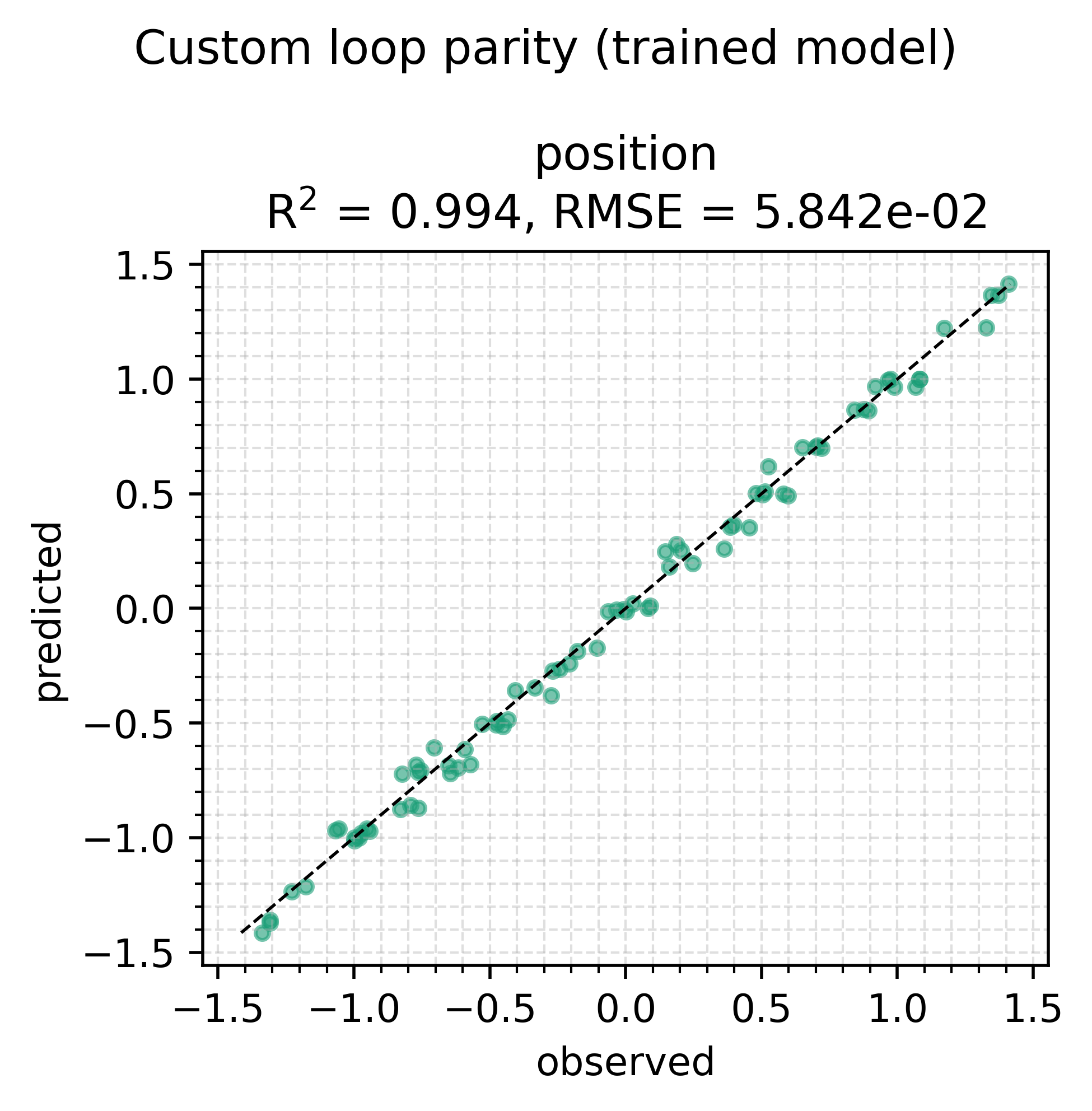
The recovered omega = 0.999 against a true 1.0 is the same accuracy the pendulum example reaches through the stock trainer — the loop is different, the physics pipeline is not.