Hybrid ODE: keep the physics, learn the gaps

One script, examples/hybrid_ode/train_hybrid_ode.py: a mechanistic model with two holes, both filled by trainable networks, every physical quantity held inside a declared range, and the measurements sampled irregularly per channel.

uv run python examples/hybrid_ode/train_hybrid_ode.py

The problem

The system is a rotation at fixed frequency $\omega$, damped at rate $k$, with a cubic coupling:

$$\frac{dy}{dt}=\left[\begin{array}{cc}-k& \omega \\ -\omega & -k\end{array}\right]y+C{y}^3,\omega =1$$

The model keeps the rotation and treats $\omega$ as known. Two things it does not know.

$k$ depends on each experiment's temperature through an Arrhenius law, running from 0.0063 to 0.276 across the six levels in the data. A factor of 44.

$C{y}^3$ is missing from the model entirely.

In a real problem you would not know either. Here they are synthesised so the fit has something to be checked against.

Two networks, two placements

	learns	called	on the solver tape
rate_net	$T\mapsto k$	once per experiment	no
residual_net	$y\mapsto$ correction	once per solver step	yes

def simulate_fn(predictors, ts, covariates, y0, solver):
    rate_net, residual_net = predictors

    # Outside the solve. One call per experiment.
    k = rate_net(covariates).reshape(())
    rotation = jnp.array([[-k, OMEGA_TRUE], [-OMEGA_TRUE, -k]])

    def vector_field(t, y, args):
        # Inside the solve. One call per solver step.
        return rotation @ y + residual_net(y)
    ...

A covariate does not change during a trajectory, so anything depending only on covariates is computed before diffeqsolve and closed over as a constant. Its cost is then independent of the step count, and it never appears on the tape the backward pass walks. A term depending on the state has to run inside.

A trainable network inside a vector field is a neural ODE. diffrax and Equinox document that technique; this example uses it in one line rather than explaining it.

The library is never told which is which. Both are ordinary calls, placed by writing the code. They travel as a plain tuple, unpacked at the top of simulate_fn, and the container is never inspected, so --mechanistic-only just shortens the tuple.

Since the residual runs inside the solve, SolverConfig gets a checkpointing adjoint. DirectAdjoint, the library default, stores the whole forward trajectory, and with a network in the vector field that is usually the memory bottleneck.

solver = SolverConfig(..., adjoint=diffrax.RecursiveCheckpointAdjoint())

Rates that span decades

rate_net maps temperature to $k$, with an output box of $({10}^{-3},1)$:

out_scaler=BoundScaler(bounds=((1e-3, 1.0),), transform="sigmoid", warp="log10")

Under linear normalisation that box has midpoint 0.5, so every rate in the data sits in the bottom 3% of the range, where the sigmoid is steepest and only large negative latents reach. A warp reparameterises the physical axis before normalising: it changes what "halfway between the bounds" means without changing which values are reachable. Under log10 the midpoint is 0.032 and the data covers the middle of the box.

The check that this worked is the fitted rate against the law it never saw:

temperature (K)	true $k$	fitted $k$	ratio
280	0.00629	0.00885	1.41
292	0.01516	0.01918	1.26
304	0.03412	0.03809	1.12
316	0.07221	0.07526	1.04
328	0.14463	0.14932	1.03
340	0.27583	0.29543	1.07

Fitted on trajectories alone, and 1.6 decades of temperature dependence come back. The worst point is the coldest, where the trajectory barely decays inside the observation window and $k$ is least identifiable.

Choosing the squash

Reparameterising costs gradient. The derivative of from_latent carries a factor ${\sigma }^{\prime }(z/T)$, and for a logistic sigmoid in float32 that factor underflows to exactly zero past $|z/T|\approx 15$. A network pushed hard against a bound stops receiving any signal to come back.

The residual is a term that visits the edge of its box early in training, so it uses softsign, whose gradient decays polynomially instead:

name	tail of $|du/dz|$	dead at
sigmoid	$e^{-|z|}$	$z\approx 17$
algebraic	$|z{|}^{-3}/2$	$z\approx 3\times {10}^3$
softsign	$|z{|}^{-2}/2$	$z\approx {10}^7$

Polynomial decay does not make saturation free. Escaping from $z=100$ under a $c/z^2$ gradient takes ${10}^6$ times as long as from $z=1$. It turns an impossible recovery into a slow one.

Registering a warp of your own

The residual's box straddles zero, so log10 is unusable, and a linear box spends resolution evenly, including on large corrections that should never happen. The script registers a signed-logarithmic axis instead, without touching the package:

from jaxhybridmodels import Warp, register_warp

register_warp(
    "symlog",
    Warp(
        forward=lambda x: jnp.sign(x) * jnp.log1p(jnp.abs(x) / SYMLOG_EPS),
        inverse=lambda w: jnp.sign(w) * SYMLOG_EPS * jnp.expm1(jnp.abs(w)),
        requires_positive=False,
    ),
)

forward(0) = 0, so the box midpoint stays at zero and a fresh residual starts near no correction rather than at some arbitrary interior point. register_bound_transform is the same idea on the squash axis.

A scaler stores its warp by name, which is what keeps a saved model a small JSON sidecar plus an array file. A custom warp therefore has to be registered before a model referencing it can be loaded.

Two data layouts, one model

--data rectangular samples every experiment on one 20-point grid with both channels measured every time:

1 bucket(s)
  bucket 0: N=24 experiments, T= 20 timestamps, D=2 channels, mask 1.00 full

--data irregular gives each experiment its own end time in $[6,9]$, its own randomly drawn sample times, and thins each channel separately to 8 or 12 samples:

3 bucket(s)
  bucket 0: N= 5 experiments, T= 15 timestamps, D=2 channels, mask 0.53 full
  bucket 1: N=11 experiments, T= 19 timestamps, D=2 channels, mask 0.53 full
  bucket 2: N= 8 experiments, T= 23 timestamps, D=2 channels, mask 0.52 full

The union length is n1 + n2 - 1 (the shared $t=0$ counts once), so with counts of 8 or 12 there are three possible lengths and therefore three buckets. Training compiles three times, nothing is padded to a common length, and nothing is dropped.

The model code is identical for both. Regular data is the degenerate case of the general one, not a separate path.

The saturation penalty

Bounds hold by construction, so a violation cannot be represented and there is nothing to clip. The failure that remains is the opposite one: a network pinned against a bound, where the squash derivative has decayed and the gradient that would pull it back has gone.

config = OptaxTrainingConfig(
    ...,
    penalty_weight=(1e-3,),   # length 1 broadcasts across phases
    penalty_points=(rate_sweep, residual_sweep),  # per leaf, in order
)

The penalty is charged on the latent, not the physical output. A penalty written against the physical value would inherit the same ${\sigma }^{\prime }(z/T)$ factor on its backward pass and die exactly where saturation is worst.

It is evaluated at the measured points — the input vectors the loss actually sees — plus any user-supplied penalty-only points. Here the residual network reads the ODE state, which the dataset cannot resolve to measured points, so both leaves are covered with a box_grid sweep (the collocation-as-extension recipe). The script prints the end-of-run value per leaf:

  end-of-run saturation penalty, by leaf:
    rate_net      3.0546e-03
    residual_net  0.0000e+00

The residual sits at exactly zero. The rate network does not, and that is the penalty working: rate_net is declared valid over 270 to 350 K, the data only reaches 340 K, and the fitted network extrapolates hard enough at the warm end to press against the top of its $k$ box. The training loss cannot see that, because no experiment is there. The trade runs both ways: a trajectory-blind penalty cannot say whether one particular solve pushed an input out of range.

Run with --penalty-weight 0 to see the term switched off.

Results

Default settings, one CPU, seeds fixed.

run	$R^2$ (y1)	$R^2$ (y2)	worst $k$ error	residual RMS
hybrid, irregular (3 buckets)	0.985	0.983	1.41x	48%
hybrid, rectangular (1 bucket)	0.979	0.976	1.81x	40%
--mechanistic-only, irregular	0.662	0.702	32.6x	n/a
--inner kan, irregular	0.990	0.992	6.40x	37%

The third row is the argument for hybrid models, and it is not the $R^2$ column that makes it. Dropping the residual leaves the rate network as the only flexible thing in the model, so it absorbs the missing cubic term into $k$ and the recovered rate goes from 1.41 times the truth at 280 K to 32.6 times. An unmodelled term does not stay in its own residual; it contaminates whichever parameter is flexible enough to absorb it, usually the one you built the experiment to measure.

The fourth row is the same effect running the other way. A KAN residual is more expressive, fits the trajectories slightly better, recovers the residual better, and recovers $k$ considerably worse, because it can absorb part of the damping too. If a fitted parameter is what you came for, the residual wants to be the least expressive thing that closes the gap.

Both data layouts reach the same trajectory accuracy, which is the point of the bucketing: half a mask is not a handicap. Their rate laws differ at the cold end because the irregular set draws end times up to 9 where the rectangular set stops at 8, and a cold experiment barely decays inside either window.

The residual RMS is measured on a grid over the data range against a true residual RMS of 0.249. It is only identifiable where trajectories went, and the grid includes corners none of them visited, so the number overstates the error the trajectory fit sees.

The default run (irregular data, MLP inner) in pictures:

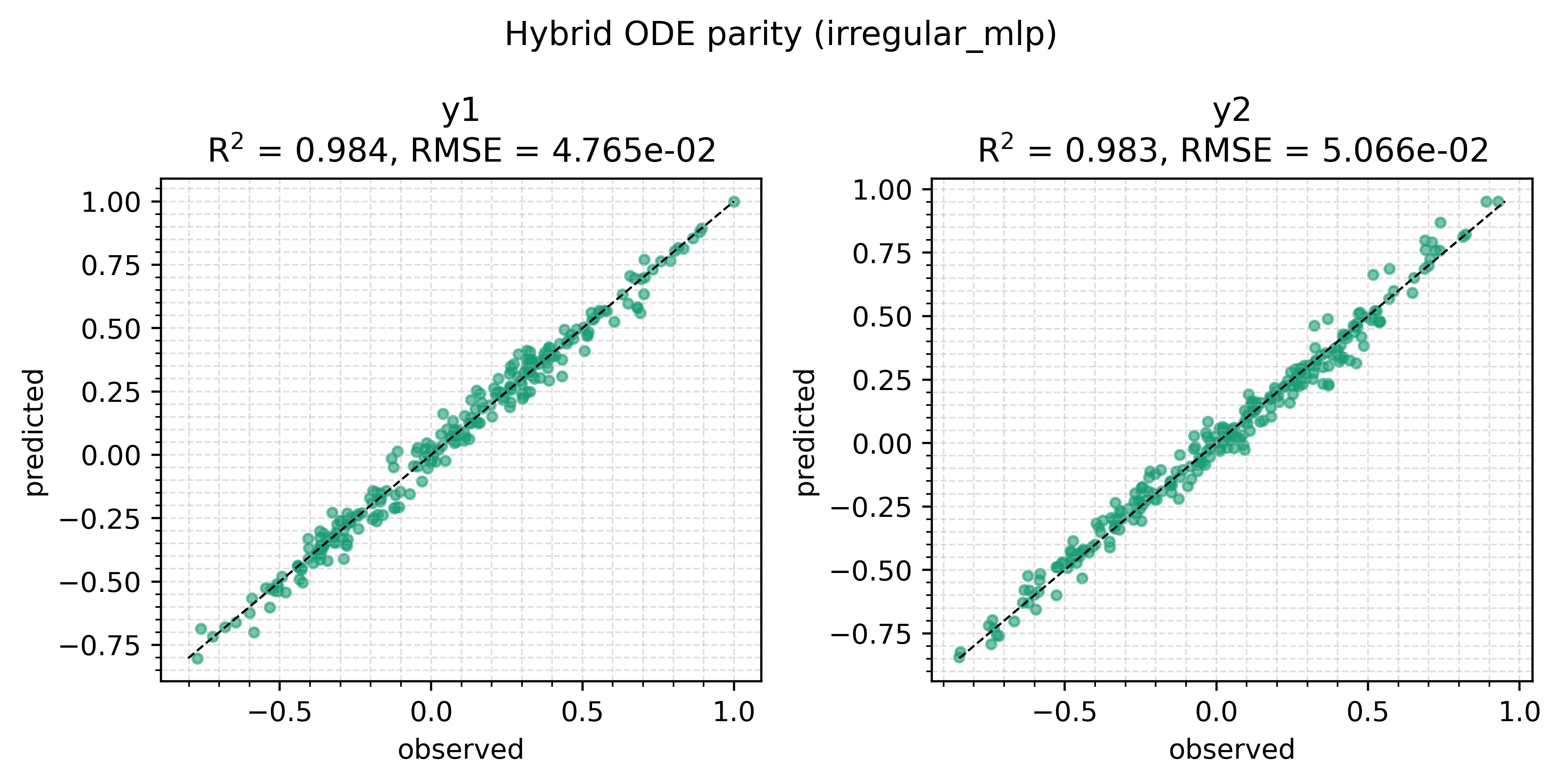
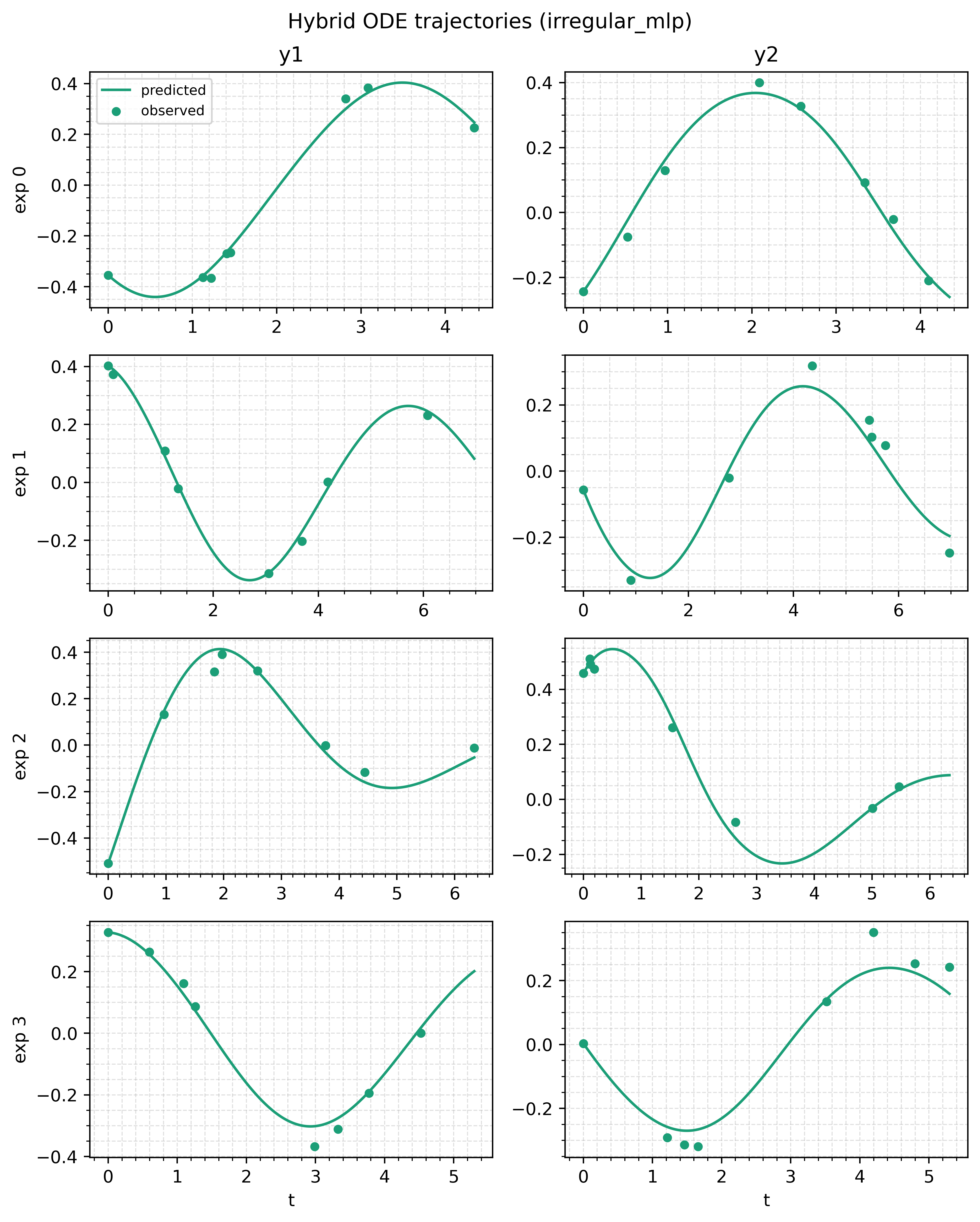
Both channels are scored only on masked-in cells; the R^2 = 0.985 / 0.983 row of the table is exactly what these two figures average.