Neural polynomial kinetics
The third predictor family alongside MLP and KAN: NeuralNPolynomial, a per-channel scalar polynomial in the (latented) input whose coefficients are produced by an inner trainable network. For crystallisation-style kinetics this is a physics-flavoured prior — a rate written as a power law in supersaturation S - 1 — instead of a black-box MLP.
The model is a two-moment crystallisation ODE
d mu0/dt =  J          (nucleation)
d mu1/dt =  G * mu0    (growth)
with growth G a known constant and nucleation J the unknown rate law. J is a NeuralNPolynomial: polynomial in supersaturation (exponents 2, 3, 4 — nucleation is strongly supersaturation driven) whose coefficients c_i(S) come from an inner MLPPredictor. The polynomial is wrapped in a BoundedPredictor so J stays in a physical range.
The dataset is synthetic: J_true(S) = a * (S - 1)^4 + b, and the fit must recover the rate law from noisy mu0 time-series across several supersaturations.
uv run python examples/supersaturation_poly/train_supersaturation_poly.pyA design fact this example surfaces
The polynomial basis is sum(inner_input) — the latented input — so NeuralNPolynomial cannot separate "coefficients from condition A" from "basis in condition B" in a single predictor. The physics-clean crystallisation form (sum_i c_i(T) * (S-1)^p_i) therefore enters either as one polynomial in S-1 with S-conditioned coefficients (shown here), or by composing two predictors. If the basis and coefficient conditions are different physical variables, write that composition explicitly at the vector-field boundary.
The script, in full
The example is a single file with no hidden parts — what you see is what runs:
"""Hybrid kinetics with a ``NeuralNPolynomial`` coefficient predictor.

The third predictor family alongside MLP and KAN: a per-channel scalar
*polynomial* in the (latented) input whose coefficients are produced by
an inner trainable network. For crystallisation-style kinetics this is a
physics-flavoured prior — a rate written as a power law in
supersaturation ``S - 1`` — instead of a black-box MLP.

Model: a two-moment crystallisation ODE

    d mu0/dt =  J          (nucleation)
    d mu1/dt =  G * mu0    (growth)

with growth ``G`` a known constant and nucleation ``J`` the unknown rate
law. ``J`` is a ``NeuralNPolynomial``: polynomial in supersaturation
(exponents ``2, 3, 4`` — nucleation is strongly supersaturation driven)
whose coefficients ``c_i(S)`` come from an inner ``MLPPredictor``. The
polynomial is wrapped in a ``BoundedPredictor`` so ``J`` stays in a
physical range.

A design fact this example surfaces: the polynomial basis is
``sum(inner_input)`` — the *latented* input — so ``NeuralNPolynomial``
cannot separate "coefficients from condition A" from "basis in condition
B" in a single predictor. The physics-clean crystallisation form
(``sum_i c_i(T) * (S-1)^p_i``) therefore enters either as one polynomial
in ``S-1`` with ``S``-conditioned coefficients (shown here), or by
composing two predictors. The latent-vs-physical basis is the open design
question (SPEC §2.3).

The dataset is synthetic: ``J_true(S) = a * (S - 1)^4 + b`` and the fit
must recover the rate law from noisy ``mu0`` time-series across several
supersaturations.

Run:
    uv run python examples/supersaturation_poly/train_supersaturation_poly.py
"""

from __future__ import annotations

import argparse
import sys
from pathlib import Path

import diffrax
import jax
import jax.numpy as jnp
import matplotlib.pyplot as plt
import numpy as np
from jax import Array

import jaxhybridmodels as hm
from jaxhybridmodels.data import ChannelObs, make_dataset, make_experiment
from jaxhybridmodels.predictors.neural_npoly import NeuralNPolynomial
from jaxhybridmodels.solver import SolverConfig

sys.path.insert(0, str(Path(__file__).resolve().parent.parent))
from _shared import (  # noqa: E402
    apply_default_style,
    parity_diagnostics,
    parity_plot,
)

# Physical truth.
G_TRUE: float = 0.1
SUPERSATURATIONS: tuple[float, ...] = (0.3, 0.6, 0.9, 1.2, 1.5)  # S - 1
T_MAX: float = 8.0
N_TIMESTEPS: int = 40
NOISE_STD: float = 0.01
J_BOUNDS: tuple[float, float] = (0.01, 2.0)
EXPONENTS: tuple[float, ...] = (2.0, 3.0, 4.0)


def true_rate(s_minus_one: float) -> float:
    """Rate law the network must learn: a power law with a small baseline."""
    return 0.02 + 0.15 * s_minus_one**4


def simulate_fn(predictors, ts, covariates, y0, solver):
    """Integrate the moment ODE with J coming from the polynomial predictor."""

    def vector_field(t, y, args):
        mu0 = y[0]
        j_rate = predictors[0](
            {"super_sat": covariates["super_sat"]}
        ).reshape(())
        return jnp.stack([j_rate, G_TRUE * mu0], dtype=jnp.float32)

    sol = solver.diffeqsolve(diffrax.ODETerm(vector_field), ts, y0)
    return jnp.asarray(sol.ys)


def state_to_output(state: Array) -> Array:
    """Only mu0 is measured."""
    return state[..., :1]


def main() -> None:
    parser = argparse.ArgumentParser(description=__doc__)
    parser.add_argument(
        "--plot-dir",
        type=Path,
        default=Path(__file__).resolve().parent / "figures",
    )
    parser.add_argument("--no-plot", action="store_true")
    args = parser.parse_args()

    apply_default_style()

    # Synthetic noisy mu0 time-series at several supersaturations.
    key = jax.random.PRNGKey(0)
    ts = jnp.linspace(0.0, T_MAX, N_TIMESTEPS)

    experiments = []
    for s_minus_one in SUPERSATURATIONS:
        key, subkey = jax.random.split(key)

        def vector_field(t_t, y, args, _s=s_minus_one):
            mu0 = y[0]
            j_rate = true_rate(_s)
            return jnp.stack([j_rate, G_TRUE * mu0])

        sol = diffrax.diffeqsolve(
            diffrax.ODETerm(vector_field),
            diffrax.Tsit5(),
            t0=ts[0], t1=ts[-1], dt0=0.05, y0=jnp.asarray([0.0, 0.0]),
            saveat=diffrax.SaveAt(ts=ts),
            stepsize_controller=diffrax.PIDController(rtol=1e-8, atol=1e-10),
            max_steps=4096,
        )
        ys = jnp.asarray(sol.ys)
        mu0_obs = ys[:, 0] + NOISE_STD * jax.random.normal(subkey, ts.shape)
        experiments.append(
            make_experiment(
                covariates={"super_sat": float(s_minus_one)},
                channels={"mu0": ChannelObs(ts=ts, values=mu0_obs)},
                y0_fn=lambda c, ch: jnp.asarray([0.0, 0.0], dtype=jnp.float32),
                exp_id=f"S_{s_minus_one:g}",
            )
        )
    ds = make_dataset(experiments, output_channel_names=("mu0",))
    print(hm.describe_buckets(ds))

    # Bounded ``NeuralNPolynomial`` rate: polynomial in S-1, coeffs from an
    # MLP. Model init and training derive from the same root key as the
    # data noise, so the whole script is reproducible from one seed.
    key, k_model, k_train = jax.random.split(key, 3)
    coeff_net = hm.MLPPredictor(
        in_size=1, out_size=len(EXPONENTS), width_size=16, depth=2,
        activation_name="tanh", key=k_model,
    )
    npoly = NeuralNPolynomial(
        coeff_net=coeff_net,
        exponents=EXPONENTS,
        in_size=1,
        out_size=1,
    )
    predictor = hm.BoundedPredictor(
        input_keys=("super_sat",),
        in_scaler=hm.BoundScaler(bounds=((-0.2, 2.0),)),
        inner=npoly,
        out_scaler=hm.BoundScaler(bounds=(J_BOUNDS,), warp="log"),
    )
    predictors = (predictor,)
    solver = SolverConfig(
        solver=diffrax.Tsit5(), rtol=1e-7, atol=1e-9, max_steps=4096, dt0=0.05,
    )
    mask = hm.trainable_mask(predictors)

    history, trained = hm.train_with_optax(
        predictors,
        ds,
        hm.OptaxTrainingConfig(
            steps=(400,),
            lr=(1e-2,),
            optimizer=("adamw",),
            reset_optimiser_state=(False,),
        ),
        simulate_fn=simulate_fn,
        state_to_output=state_to_output,
        solver=solver,
        trainable=mask,
        key=k_train,
    )

    preds = hm.predict_dataset(
        trained, ds, simulate_fn=simulate_fn,
        state_to_output=state_to_output, solver=solver,
    )
    hm.print_metrics(
        hm.compute_metrics(preds, ds), header=f"fit (final data loss {history[-1]:.3e})"
    )

    # The recovered rate law vs truth.
    print("\nrecovered J(S) vs truth:")
    for s_minus_one in SUPERSATURATIONS:
        learned = hm.evaluate_predictor(trained[0], {"super_sat": s_minus_one})
        truth = true_rate(s_minus_one)
        print(f"  S-1={s_minus_one:4.1f}  J_learned={learned:.4f}  J_truth={truth:.4f}")

    if not args.no_plot:
        args.plot_dir.mkdir(parents=True, exist_ok=True)
        # ``compute_metrics`` keeps only the summary stats; the scatter needs
        # the raw value pairs, so re-walk the mask here.
        parity_data = parity_diagnostics(preds, ds)
        parity_plot(
            parity_data,
            title="Neural polynomial kinetics parity (trained model)",
            save_path=args.plot_dir / "parity.png",
        )

        # The recovered rate law against the truth it had to find.
        fig, ax = plt.subplots(figsize=(6.4, 4.2))
        s = np.asarray(SUPERSATURATIONS)
        learned = np.asarray(
            [
                float(hm.evaluate_predictor(trained[0], {"super_sat": float(v)}))
                for v in SUPERSATURATIONS
            ]
        )
        truth = np.asarray([true_rate(v) for v in SUPERSATURATIONS])
        dense = np.linspace(s[0], s[-1], 200)
        ax.plot(dense, [true_rate(v) for v in dense], color="black", ls="--", lw=1.4, label="truth")
        ax.plot(s, learned, color="tab:red", marker="o", lw=1.4, label="learned J(S)")
        ax.set_xlabel("supersaturation  S − 1")
        ax.set_ylabel("nucleation rate  J")
        ax.set_title("Recovered rate law")
        ax.legend(fontsize=8)
        fig.tight_layout()
        fig.savefig(args.plot_dir / "recovered_rate.png")
        plt.close(fig)
        print(f"\n[plot] figures written to {args.plot_dir}")


if __name__ == "__main__":
    main()
Results
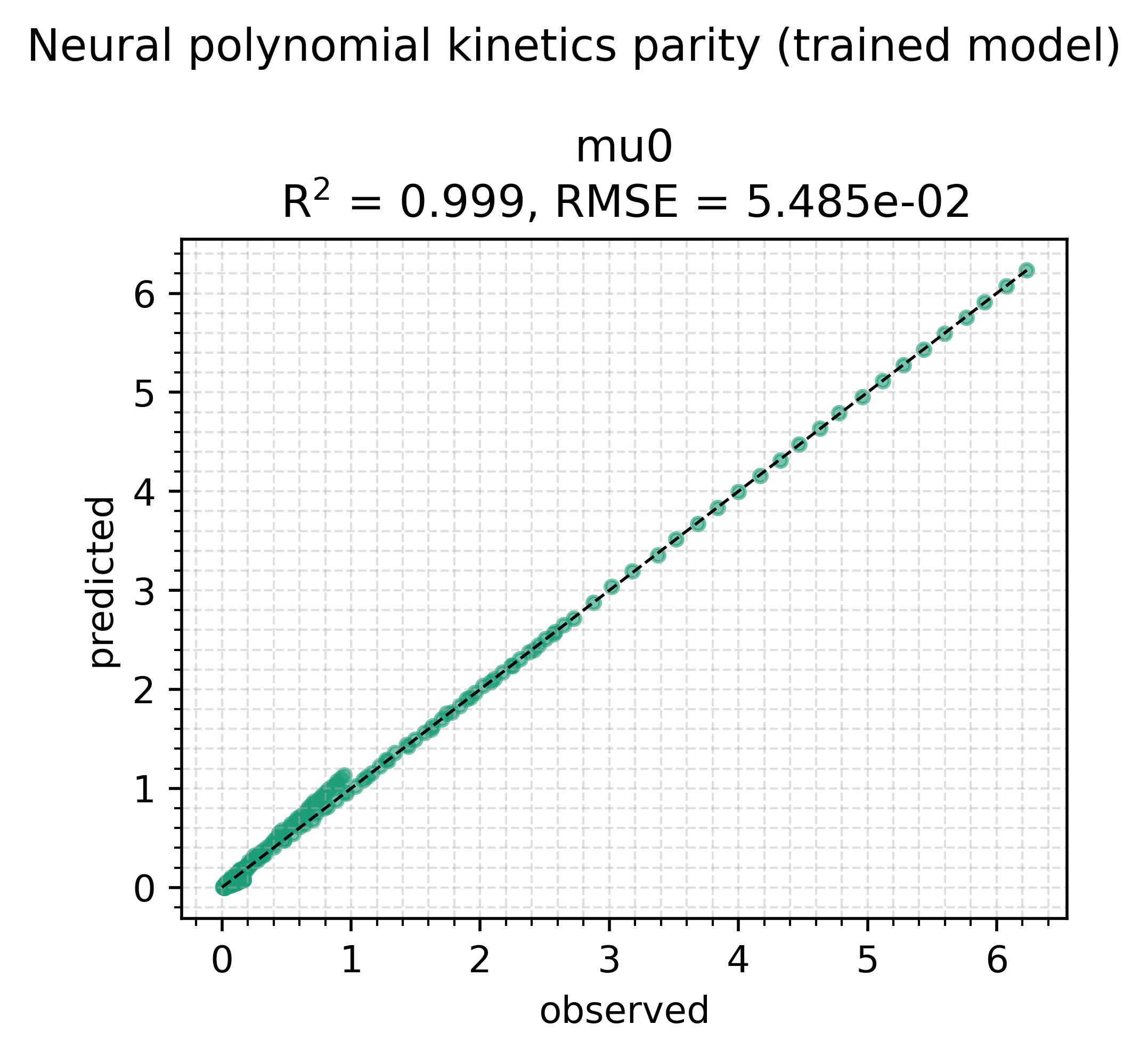
Default settings, seed 0, 400 steps. The mu0 time-series fit to the noise floor (R^2 = 0.999), and the rate law comes out close to the truth J(S) = 0.02 + 0.15 (S-1)^4.
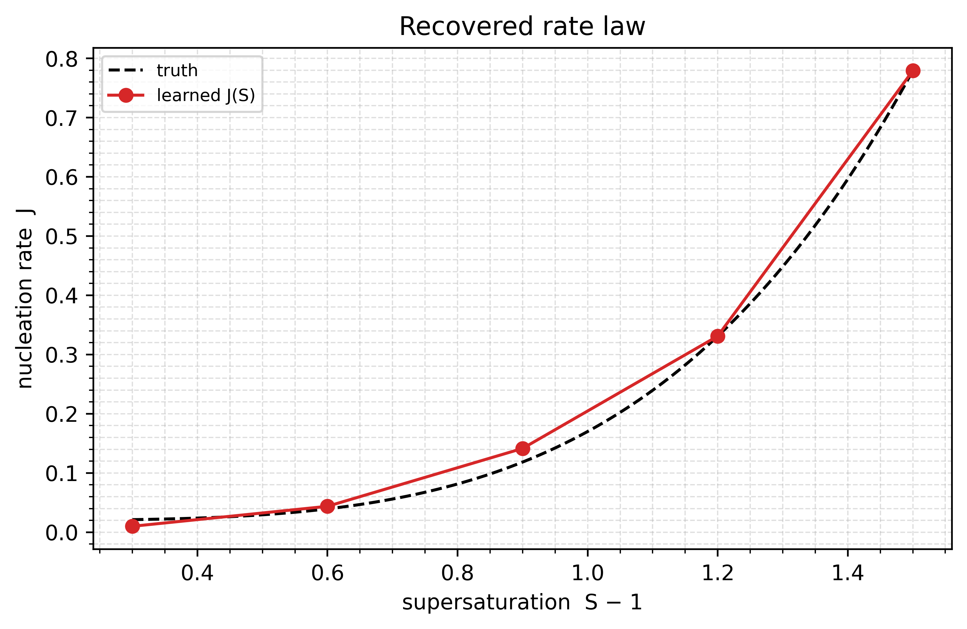
The recovered curve is a polynomial in the latented input wrapped in a BoundedPredictor's output scaler, so the shape is the network's and the range is structural. The fit is best at high supersaturation, where nucleation actually drives the observable dynamics.