Crystallisation (hybrid MLP)

The canonical end-to-end example: a hybrid kinetic model fitted to four crystallisation experiments, each an irregular concentration trajectory with one particle-size measurement at the end. Two neural networks emit the unknown rate laws, and those rates drive a population-balance ODE.

Crystallisation is a dissolved solute leaving solution as solid crystals, driven by nucleation, new crystals appearing, and growth, existing ones getting larger. Nobody can derive either rate from first principles for a given system, which is the situation this library is for.

The full script is examples/crystallisation/train_kinetic.py:

bash

uv run python examples/crystallisation/train_kinetic.py

The four experiments are written into it, so there is no external data dependency. Every section here matches a section of the file.

What we're modelling

A six-state population balance:

\begin{aligned} \frac{d μ_{0}}{d t} & = J (t) \\ \frac{d μ_{k}}{d t} & = k G (t) μ_{k - 1}, k = 1, 2, 3, 4 \\ \frac{d conc}{d t} & = - 3 K_{v} ρ_{c} G (t) μ_{2} \end{aligned}

The $μ_{k}$ are moments of the crystal size distribution: $μ_{0}$ counts crystals, $μ_{3}$ tracks total volume, and $μ_{4} / μ_{3}$ gives a mean diameter. Tracking five moments instead of the full distribution turns a partial differential equation into six ordinary ones.

$G$ (growth velocity, m/s) and $J$ (nucleation rate, per m³ per second) are the unknowns. Rather than commit to Classical Nucleation Theory or a power law, two networks learn $\log_{10} G$ and $\log_{10} J$ from (temperature_C, supersaturation), and the vector field exponentiates back to physical rates inside the integrator. Supersaturation is concentration over saturation concentration; above 1 the solution is loaded and crystals can form.

Two quantities are observed: concentration (measured often) and the volume-weighted mean diameter $d_{43} = μ_{4} / μ_{3} \cdot 10^{6}$ µm (one measurement per experiment, at the end).

For a parametric counterpart that fits four scalars instead of two networks, see Crystallisation (mechanistic).

The dataset

Four experiments reproduced from the thesis Unseeded_LowData4 cut, rounded to 1 dp on values and 3 dp on variance. Concentration variance is one made-up scalar (CONC_VAR = 0.1) broadcast across every row. The $d_{43}$ variances are the rounded thesis values.

`exp_id`	T (°C)	n conc	n d43	t span (min)	terminal d43 (µm)
`LowData4_3`	17.0	9	1	0 → 270	9.2
`LowData4_4`	17.0	9	1	0 → 270	7.7
`LowData4_7`	21.0	7	1	0 → 360	10.5
`LowData4_9`	21.0	7	1	0 → 375	11.9

Two experiments at each of two temperatures, on different time grids. make_dataset merges each experiment's per-channel timestamps into one axis and groups by that axis's length, so training sees two groups.

Step 1: define the experiments

An experiment is one run of the real thing. A channel is one measured quantity with its own timestamps. A covariate is a condition that stays fixed for the whole run.

python

from jaxhybridmodels import ChannelObs, Experiment, make_experiment

EXPERIMENTS_DATA = (
    {
        "exp_id": "LowData4_3",
        "temperature_C": 17.0,
        "time_min": (0.0, 30.0, 60.0, 90.0, 120.0, 150.0, 180.0, 225.0, 270.0),
        "conc": (14.7, 13.7, 7.7, 7.0, 5.7, 5.5, 5.4, 5.1, 5.2),
        "d43_time_min": 270.0,
        "d43": 9.2,
        "d43_var": 5.345,
    },
    # ... three more entries (LowData4_4, _7, _9), see the script
)
CONC_VAR = 0.1  # made-up uniform concentration variance, broadcast per row

def y0_fn(covariates, channels):
    """Initial state [mu0..mu4, conc]: moments at zero, conc at first observation."""
    init_conc = jnp.asarray(channels["conc"].values[0])
    return jnp.concatenate([jnp.zeros(5, dtype=init_conc.dtype), init_conc[None]])

experiments = []
for data in EXPERIMENTS_DATA:
    time_min = jnp.asarray(data["time_min"], dtype=float)
    conc = jnp.asarray(data["conc"], dtype=float)
    experiments.append(make_experiment(
        covariates={"temperature_C": float(data["temperature_C"])},
        channels={
            "conc": ChannelObs(
                ts=time_min, values=conc,
                variance=jnp.full_like(conc, CONC_VAR),
            ),
            "d43": ChannelObs(
                ts=jnp.asarray((data["d43_time_min"],), dtype=float),
                values=jnp.asarray((data["d43"],), dtype=float),
                variance=jnp.asarray((data["d43_var"],), dtype=float),
            ),
        },
        y0_fn=y0_fn,
        exp_id=str(data["exp_id"]),
    ))

y0_fn builds the ODE's full initial state. It runs once per experiment, when you build it, never during training. Five moments start at zero, because the suspension is nominally clear at t = 0. Concentration starts at the first observed value. Temperature is the only covariate; the thesis Loading column is uniformly zero across LowData4 and is dropped on purpose.

The two channels carry independent time axes. conc has 7 to 9 points per experiment; d43 has one, at the end. make_dataset recovers that sparsity without any mask code from you.

Step 2: the state_to_output projector

The integrator returns all six states. We observe two. state_to_output maps one to the other, and here it also derives $d_{43}$ from two moments.

python

D43_MU3_EPS = 1e-6
D43_MAX = 55.0

def state_to_output(state):
    """[T, 6] -> [T, 2] in OUTPUT_CHANNELS = ('conc', 'd43') order."""
    mu3, mu4, conc = state[..., 3], state[..., 4], state[..., 5]
    safe_mu3 = jnp.where(mu3 > D43_MU3_EPS, mu3, 1.0)
    ratio = jnp.where(mu3 > D43_MU3_EPS, (mu4 / safe_mu3) * 1e6, 0.0)
    d43 = jnp.clip(jnp.where(jnp.isfinite(ratio) & (ratio > 0.0), ratio, 0.0), 0.0, D43_MAX)
    return jnp.stack([conc, d43], axis=-1)

The safe_mu3 line is mandatory, not stylistic: replacing the divisor before dividing is what keeps the gradient finite on the discarded branch. See Recommendations.

Step 3: build the dataset

python

from jaxhybridmodels import describe_buckets, make_dataset

dataset = make_dataset(experiments, output_channel_names=("conc", "d43"))
print(describe_buckets(dataset))

Two buckets. The 17 °C pair merge to length 9, since d43_time_min=270 already sits in the concentration grid; the 21 °C pair to length 7, their d43 times each already sitting in the concentration grid. Each bucket compiles once and is reused for the whole run.

Step 4: two bounded predictors

The convention is a tuple: (growth_bp, nucleation_bp). Both take the same two-key dict, and each BoundedPredictor picks out the keys named in its input_keys.

MLP and KAN side by side

The shipped script trains the same (growth_bp, nucleation_bp) structure twice, once with an MLPPredictor inside and once with a KANPredictor, writing figures into figures/mlp/ and figures/kan/. The walkthrough below shows the MLP path. The KAN swap is one line: replace MLPPredictor(...) with KANPredictor(in_size=2, out_size=1, hidden_widths=(64,), grid_size=5, basis="spline", key=...). Bounds, scalers, and the surrounding ODE are identical.

python

from jaxhybridmodels import BoundedPredictor, BoundScaler, MLPPredictor

INPUT_KEYS = ("temperature_C", "supersaturation")
TEMPERATURE_BOUNDS = (13.0, 27.0)        # °C, slightly wider than data span
SUPERSATURATION_BOUNDS = (0.0, 12.0)     # S = conc / conc_sat
LOG10_GROWTH_BOUNDS = (-15.0, -5.0)      # log10(G [m/s])
LOG10_NUCLEATION_BOUNDS = (-6.5, 20.0)   # log10(J [#/(m^3·s)])

in_scaler = BoundScaler(
    bounds=(TEMPERATURE_BOUNDS, SUPERSATURATION_BOUNDS),
    transform="sigmoid",
)

k_growth, k_nucleation = jr.split(key, 2)

growth = BoundedPredictor(
    input_keys=INPUT_KEYS,
    in_scaler=in_scaler,
    inner=MLPPredictor(in_size=2, out_size=1, width_size=64,
                       depth=1, activation_name="relu", key=k_growth),
    out_scaler=BoundScaler(bounds=(LOG10_GROWTH_BOUNDS,), transform="sigmoid"),
)
nucleation = BoundedPredictor(
    input_keys=INPUT_KEYS,
    in_scaler=in_scaler,
    inner=MLPPredictor(in_size=2, out_size=1, width_size=64,
                       depth=1, activation_name="relu", key=k_nucleation),
    out_scaler=BoundScaler(bounds=(LOG10_NUCLEATION_BOUNDS,), transform="sigmoid"),
)

predictors = (growth, nucleation)

The bound choice matters more than anything else on this page. A fresh network emits the midpoint of its output box, so that is what the integrator sees on step 0. LOG10_GROWTH_BOUNDS = (-15, -5) puts it at $G \approx 10^{- 10}$ m/s, reasonable for early growth. An earlier (-12, -3) draft put it at $G \approx 3 \cdot 10^{- 8}$ m/s, large enough that random weights produced rates the moment solver could not track within max_steps. See Recommendations.

Optional: pin the readout to the box midpoint

The nucleation box spans 26 decades, so even well centred an unlucky readout draw can start far enough off midpoint to make the ODE intractably stiff. MLPPredictor.with_zero_final_head() and its KAN counterpart zero the readout layer, putting the initial output exactly at the midpoint whatever the key. Hidden layers keep their random init.

python

inner=MLPPredictor(in_size=2, out_size=1, width_size=64,
                   depth=1, activation_name="relu", key=k_growth).with_zero_final_head()

The shipped script runs without it on the default seed. Turn it on if you hit max_steps on another.

Step 5: the vector field

This is where you write physics. The simulate_fn signature is fixed. Everything inside it is yours.

python

RHO_C = 1370.0    # crystal density [kg/m^3]
K_V = 0.81        # volumetric shape factor
META_EPS = 1e-5   # supersaturation must exceed 1 + eps for nucleation/growth

def simulate_fn(predictors, ts, covariates, y0, solver):
    growth_bp, nucleation_bp = predictors
    temperature_C = covariates["temperature_C"]
    # Empirical solubility polynomial in °C.
    conc_sat = (0.3705 + 7.171e-2 * temperature_C
                - 1.924e-3 * temperature_C**2
                + 17.97e-5 * temperature_C**3)

    def vector_field(t, y, args):
        mu0, mu1, mu2, mu3, _mu4, conc = y[0], y[1], y[2], y[3], y[4], y[5]
        S = conc / conc_sat

        # Predictor inputs. Temperature is a covariate, constant in time;
        # supersaturation comes from the state and changes every step.
        # The library treats every key as a named scalar either way.
        inputs = {"temperature_C": temperature_C, "supersaturation": S}

        meta_mask = (S > 1.0 + META_EPS).astype(y.dtype)
        log10_G = jnp.squeeze(growth_bp(inputs))
        log10_J = jnp.squeeze(nucleation_bp(inputs))
        G = meta_mask * jnp.power(10.0, log10_G)
        J = meta_mask * jnp.power(10.0, log10_J)

        return jnp.stack([
            J,                                 # dmu0
            G * mu0,                           # dmu1
            2.0 * G * mu1,                     # dmu2
            3.0 * G * mu2,                     # dmu3
            4.0 * G * mu3,                     # dmu4
            -3.0 * K_V * RHO_C * G * mu2,      # dconc
        ])

    times_sec = ts * 60.0  # dataset stores minutes; rate constants are SI seconds.
    sol = diffrax.diffeqsolve(
        diffrax.ODETerm(vector_field), solver.solver,
        t0=times_sec[0], t1=times_sec[-1], dt0=solver.dt0, y0=y0,
        saveat=diffrax.SaveAt(ts=times_sec),
        stepsize_controller=solver.stepsize_controller(),
        max_steps=solver.max_steps,
        adjoint=solver.adjoint,
    )
    return jnp.asarray(sol.ys)

Two notes. The metastable mask zeros both rates below $S = 1 + 10^{- 5}$ , so the ODE stops moving once the solution is no longer loaded. And the time conversion is one line, because keeping the dataset in minutes makes the plots readable.

solver.stepsize_controller() and solver.adjoint come from the SolverConfig. Building a PIDController by hand instead would silently ignore a per-state atol tuple.

Step 6: solver and training config

The moments span roughly 18 decades during an integration, so atol gets one entry per state component.

python

from jaxhybridmodels import OptaxTrainingConfig, SolverConfig, train_with_optax

solver = SolverConfig(
    solver=diffrax.Tsit5(),
    rtol=1e-4,
    atol=(1e3, 1e-2, 1e-6, 1e-10, 1e-14, 1e-5),  # about 9 decades below each natural magnitude
    max_steps=500_000,
    dt0=None,
)

config = OptaxTrainingConfig(
    steps=(600,),
    lr=(1e-3,),
    optimizer=("adamw",),
    reset_optimiser_state=(False,),
    length_schedule=(1.0,),
    loss="mse",
    verbose=True,
)

One phase to start. Add a second at a lower learning rate once the loss flattens.

Step 7: train

python

history, trained_predictors = train_with_optax(
    predictors, dataset, config,
    simulate_fn=simulate_fn, state_to_output=state_to_output,
    solver=solver, key=jr.PRNGKey(0),
)
print(f"final loss: {history[-1]:.6f}")

The first step pays for compilation, once per bucket shape. Every step after that runs at full speed.

Step 8: predict and inspect

python

from jaxhybridmodels import predict_dataset

predictions = predict_dataset(
    trained_predictors, dataset, simulate_fn=simulate_fn,
    state_to_output=state_to_output, solver=solver,
)
# One [N, T, D] array per bucket, in the same order as dataset.bucket_payloads.
# The buckets differ in T, so they cannot be stacked into one tensor.

# Read the trained rate laws at any condition you like.
sample_inputs = {
    "temperature_C": jnp.asarray(20.0),
    "supersaturation": jnp.asarray(1.5),
}
trained_growth, trained_nucleation = trained_predictors
log10_G = float(jnp.squeeze(trained_growth(sample_inputs)))
log10_J = float(jnp.squeeze(trained_nucleation(sample_inputs)))
print(f"G(20°C, S=1.5) = {10**log10_G:.2e} m/s, J = {10**log10_J:.2e} #/(m³·s)")

Reading the predictors at conditions no experiment visited is the point of a bounded hybrid model. The script also writes parity and trajectory plots under examples/crystallisation/figures/.

Default settings, seed 0, 600 steps for the MLP family:

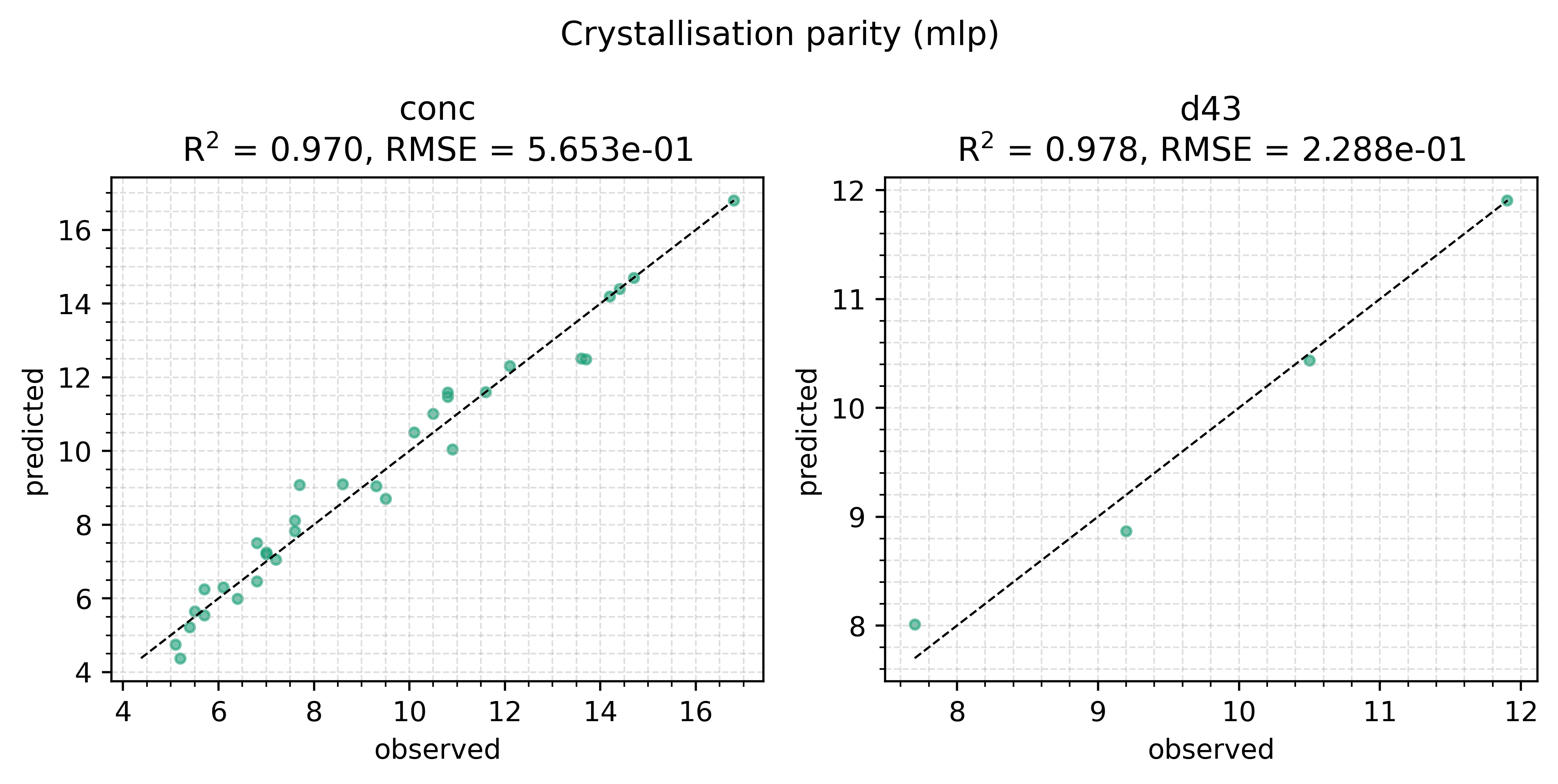
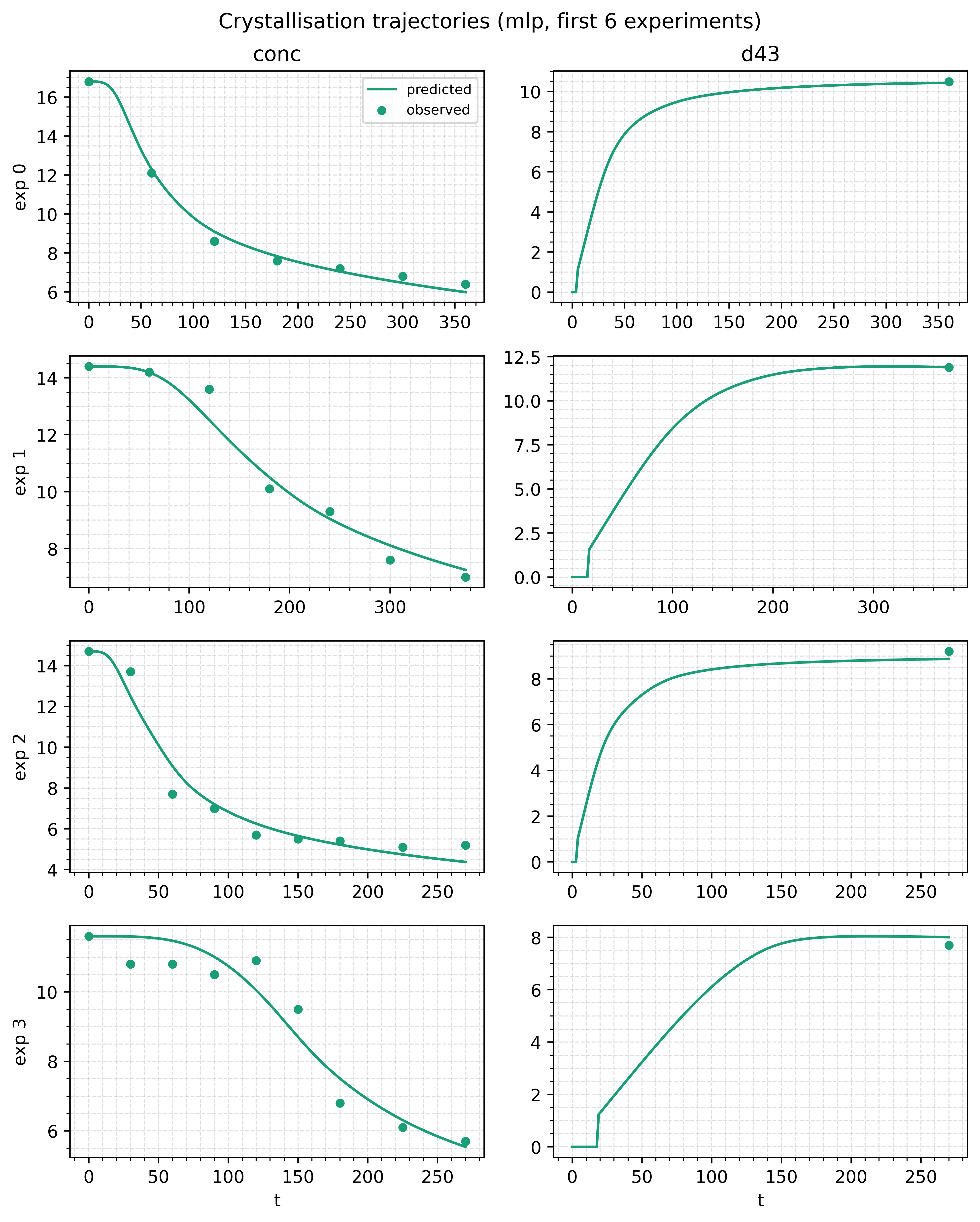
Predicted against observed concentration and d43

Fitted trajectories against the four experiments

The concentration parity sits close to the identity line across the full concentration range, and the terminal d43 points land within their variance of the fitted curves. The KAN family (--kan-basis spline defaults) reaches a similar concentration fit but recovers the d43 terminal size worse, which is the same least-expressive-model lesson the hybrid ODE and custom predictor examples show.

Crystallisation (hybrid MLP) ​

What we're modelling ​

The dataset ​

Step 1: define the experiments ​

Step 2: the state_to_output projector ​

Step 3: build the dataset ​

Step 4: two bounded predictors ​

Step 5: the vector field ​

Step 6: solver and training config ​

Step 7: train ​

Step 8: predict and inspect ​

Crystallisation (hybrid MLP)

What we're modelling

The dataset

Step 1: define the experiments

Step 2: the state_to_output projector

Step 3: build the dataset

Step 4: two bounded predictors

Step 5: the vector field

Step 6: solver and training config

Step 7: train

Step 8: predict and inspect