Custom predictor: a predictor family of your own

The library ships an MLP and a KAN, but a predictor is only a trainable module mapping an array to an array. This example writes a third family from scratch and trains it inside a hybrid ODE. The framework never learns that it is not an MLP.

The script lives at examples/custom_predictor/train_custom_predictor.py. Run it with:

uv run python examples/custom_predictor/train_custom_predictor.py

The data is synthesised on every run, so there is no file to manage. The procedure this example follows is written up in Custom predictors.

The problem

First-order decay whose rate depends on temperature:

$$\frac{dy}{dt}=-k(T)y,k(T)=A\exp (-\frac{E_a}{RT})$$

Each experiment is one isothermal run: a temperature between 290 and 350 K, a decay curve of 15 noisy points, and the same initial concentration $y_0=1$. All runs share a timestamp grid, so the dataset is one fully observed bucket.

The Arrhenius form on the right is the answer, not an input. The predictor sees a temperature and must produce a rate. The true rates run from 0.029 to 0.998, which is 1.5 decades, so the output scaler warps logarithmically.

The predictor: random Fourier features

Random Fourier features project the input through a fixed random bank of cosines, then fit linear weights on top:

$$\varphi (x)=\sqrt{\frac{2}{m}}\cos (x\mathrm{\Omega }+b),f(x)=\varphi (x)W+c$$

The bank $(\mathrm{\Omega },b)$ is drawn once and never updated. Only the readout $(W,c)$ learns. That is what makes this random features rather than a one-hidden-layer network with a cosine activation.

class RandomFourierPredictor(Predictor):
    weights: Float[Array, "n_features out_size"]      # trainable
    bias: Float[Array, " out_size"]                   # trainable
    frequencies: Float[Array, "in_size n_features"]   # fixed bank
    phases: Float[Array, " n_features"]               # fixed bank
    in_size: int = eqx.field(static=True)
    out_size: int = eqx.field(static=True)
    n_features: int = eqx.field(static=True)
    bandwidth: float = eqx.field(static=True)

    def __call__(self, x):
        features = jnp.sqrt(2.0 / self.n_features) * jnp.cos(x @ self.frequencies + self.phases)
        return features @ self.weights + self.bias

The split between trained and fixed arrays is the reason this architecture was chosen for the example. It forces every question the contract asks, and the next four sections are the four answers.

Which fields are static

in_size, out_size, n_features, and bandwidth are eqx.field(static=True). They are shape and configuration, the optimiser never sees them, and they are not written to the checkpoint. The four arrays are ordinary fields and are written.

bandwidth is the standard deviation of the frequency draw. It sets the length scale the features can resolve. Because BoundScaler hands the inner predictor a latent input of roughly unit scale, a bandwidth near 1 is the sane starting point regardless of what the covariate's physical units are. --bandwidth changes it.

How it re-initialises

The run uses a three-attempt restart tournament, so the module has to be able to produce fresh weights. initialized_with_key rebuilds it through __init__:

def initialized_with_key(self, key: Array) -> RandomFourierPredictor:
    return RandomFourierPredictor(
        in_size=self.in_size, out_size=self.out_size,
        n_features=self.n_features, bandwidth=self.bandwidth, key=key,
    )

Leave it out and the default resamples all four arrays from a standard normal. The phases would no longer be uniform on $[0,2\pi )$, the readout would lose its $1/\sqrt{m}$ scaling, and bandwidth would be ignored. Shapes are unchanged by the rebuild, which matters: the trainability mask is built before training and reused after a restart.

How the bank is held fixed

A module cannot declare its own field untrainable. Trainability is a boolean mask over the pytree, built by the caller:

BANK_PATHS = ("0.inner.frequencies", "0.inner.phases")

mask = trainable_mask(predictors)
mask = freeze_paths(mask, BANK_PATHS)

The paths read from the root of the predictors tuple: element 0, its inner, its frequencies. freeze_paths raises on a path that matches no leaf, so renaming a field fails loudly instead of quietly training an array you believed was fixed.

--train-bank skips the freeze, which turns the model into an ordinary cosine-activation network. The results table below has both.

How it round-trips

The script saves and reloads the trained predictor before reporting diagnostics, and prints the largest change in the learned rate. It is 0.000e+00.

Loading needs a template with the same class, container shape, and static fields, which the script builds by calling the same _build_predictor used for training. That is the whole reason to keep static fields to plain scalars: you have to be able to reproduce them at the load site.

Bounds stay outside

RandomFourierPredictor contains no bound, no covariate name, and no unit. The wrapper supplies all three:

BoundedPredictor(
    input_keys=("temperature",),
    in_scaler=BoundScaler(bounds=((280.0, 360.0),), transform="sigmoid"),
    inner=RandomFourierPredictor(in_size=1, out_size=1, ...),
    out_scaler=BoundScaler(bounds=((1e-2, 3.0),), transform="sigmoid", warp="log10"),
)

The input box is wider than the sampled temperatures so the scaler stays clear of its saturating ends. The output box is loose on purpose: under a log10 warp, headroom costs almost no resolution.

Where the predictor sits

The rate is constant along a trajectory, so simulate_fn calls the predictor once, above diffeqsolve, and the network never touches the solver tape:

def _simulate_fn(predictors, ts, covariates, y0, solver):
    (rate,) = predictors
    k = rate(covariates).reshape(())

    def vector_field(t, y, args):
        return -k * y
    ...

See Where a predictor sits relative to the solver for the case where it cannot.

Results

Default settings, seed 0, 400 steps after the tournament. "Worst rate error" is the largest relative error in $k(T)$ across the seven sampled temperatures.

run	final data loss	$R^2$	worst rate error
default: 64 features, bandwidth 1, bank frozen	8.68e-05	0.9992	1.26%
--n-features 16	8.60e-05	0.9992	1.54%
--train-bank	8.52e-05	0.9992	1.97%
--bandwidth 8	8.44e-05	0.9993	3.34%

Every row fits the trajectories to the noise floor, and the ranking on trajectory loss is the reverse of the ranking on the rate law. The wigglier and freer the basis, the better it fits 105 noisy points and the worse it recovers $k(T)$. The errors concentrate at 340 and 350 K, the edge of the sampled range, where a flexible basis is least constrained.

That is the same trade the hybrid ODE example shows with a KAN residual. If a physical quantity is what you came for, the predictor wants to be the least expressive thing that fits.

Sixteen features are enough here because the target is one smooth monotone curve. The default is 64 to leave room for a harder rate law.

The default run (64 features, bank frozen) in pictures:

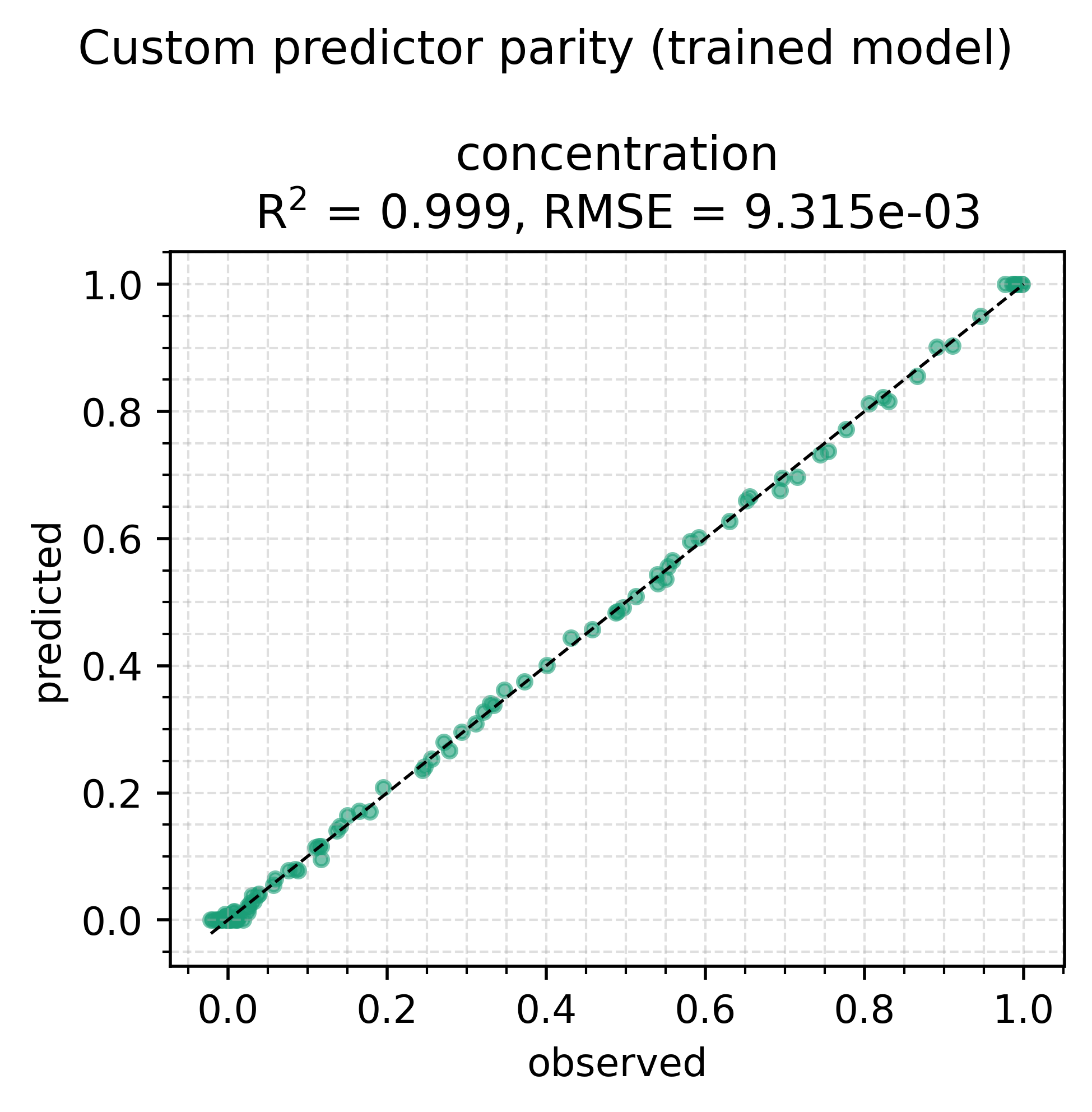
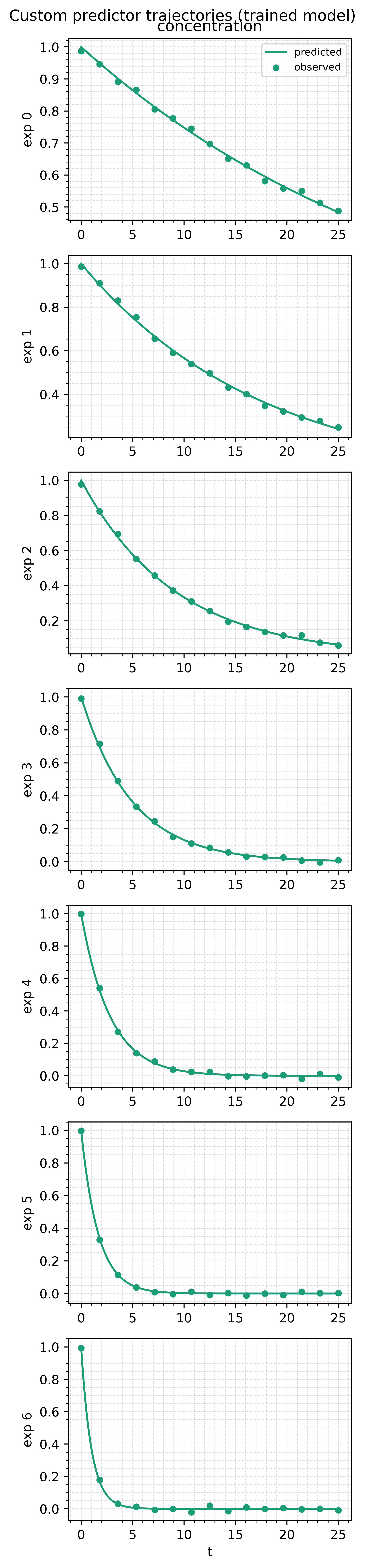
The parity scatter is noise-floor tight, and the trajectories show the fit's worst point: the two coldest runs (least decay in the window), where the rate law's relative error concentrates.