Multiple shooting
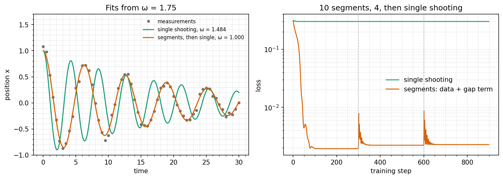
A fit can fail because the optimiser can't see where to go, even when the model is right. Here a damped oscillator's frequency is fitted from a poor guess. Single shooting settles on the wrong answer. Splitting the trajectory into segments finds the right one, and the schedule ends in single shooting, so the returned model is an ordinary one.
Read the multiple shooting section of the training guide for the settings.
Run it
uv run python examples/multiple_shooting/oscillator.py
uv run python examples/multiple_shooting/oscillator.py --no-plot
About 40 seconds on CPU. It prints the fitted frequency from three starts and the segmented run's summary, and writes multiple_shooting.png to examples/multiple_shooting/figures/.
The model
The state is
def simulate_fn(predictors: Any, ts: Any, covariates: Any, y0: Any, solver: Any) -> Any:
    w = predictors["w"].value

    def field(t: Any, y: Any, args: Any) -> Any:
        return jnp.stack([y[1], -(w**2) * y[0] - DAMPING * y[1]])

    return solver.diffeqsolve(diffrax.ODETerm(field), ts, y0)


def oscillator(frequency: float) -> hm.HybridModel:
    """The model at a starting frequency; the state is ``(x, v)`` and only ``x`` is measured."""
    return hm.HybridModel(
        predictors={"w": hm.Parameter(frequency, bounds=(0.1, 3.0))},
        simulate_fn=simulate_fn,
        state_to_output=lambda state: state[:, :1],
        output_channel_names=("x",),
    )
Why single shooting fails
From
Segments, then single shooting
Each schedule runs 900 steps:
SINGLE = hm.OptaxTrainingConfig(steps=900, lr=0.03)
SEGMENTED = hm.OptaxTrainingConfig(
    phases=(
        hm.TrainingPhase(steps=300, lr=0.03, shooting_segments=10),
        hm.TrainingPhase(steps=300, lr=0.03, shooting_segments=4),
        hm.TrainingPhase(steps=300, lr=0.03),  # segments=1: single shooting
    )
)
Ten segments of seven samples each, sharing one sample with the next, span 3 time units: half a cycle at the true frequency, and 0.84 of one at the starting guess of 1.75. That is how long a wrong frequency has to go wrong before the next segment starts afresh from its own node. Four segments follow, then single shooting:
Fitted frequency (truth 1.0), 900 steps each:
  start    single  segmented
   0.40    1.0000     1.0000
   1.75    1.4840     1.0000
   1.95    1.4841     1.0000
The summary's phase table shows the gap term, the cost of the joins not meeting, at the end of each segmented phase:
Phases
  phase  steps    first loss     last loss  last gap term
      0    300    3.1133e-01    1.7887e-03     1.4489e-04
      1    300    2.2790e-03    2.1804e-03     3.9050e-05
      2    300    2.2786e-03    2.2767e-03              -
The loss spikes briefly at steps 300 and 600, where the optimiser restarts for the new segment count.
When it is not enough
Segments have to be short compared with how fast the model moves at its starting guess, well under a cycle each here. On these data, ten segments also recover
Some models never need segments. With the damping also fitted, single shooting reaches