Tubular reactor

A reaction rate learned inside a partial differential equation. The tube is discretised into 50 cells, so the model state has 50 entries, but only four sensors are measured. The example shows that a PDE needs nothing special from the library: the method of lines turns it into an ODE, simulate_fn returns the whole field, and state_to_output picks the sensor cells.

Read it after the hybrid ODE example, which covers networks inside the vector field on a small state.

Run it

uv run python examples/tubular_reactor/train_tubular_reactor.py
uv run python examples/tubular_reactor/train_tubular_reactor.py --steps 5 --no-plot  # smoke test

About two minutes on CPU at the default 600 steps per model. Prints both fits' metrics and the learned rate against the truth, and writes sensors.png, rate_law.png and field.png to examples/tubular_reactor/figures/.

The model

Liquid flows through a tube of length $L=1$ at speed $u=1$, with axial dispersion $D=0.01$, and a reactant is consumed as it goes:

$$\frac{\partial c}{\partial t}=-u\frac{\partial c}{\partial z}+D\frac{{\partial }^{2}c}{\partial z^2}-r(c,T)$$

The inlet concentration is held at the feed value, which drops to 30% at $t=1.5$; the outlet has zero gradient. Advection uses first-order upwind differences and dispersion central differences. Each of the six experiments has its own temperature $T$ and feed concentration, both covariates.

Transport is known. The rate law is not. The data come from Langmuir-Hinshelwood kinetics,

$$r=\frac{k(T)c}{1+Kc},k(T)=k_{\text{ref}}\exp (-\frac{E_a}{R}(\frac{1}{T}-\frac{1}{T_{\text{ref}}})),$$

with $E_a/R=4000$ K and $K=2$. The hybrid model writes $r=g(c,T)c$ and learns $g$ with a bounded network. Factoring out $c$ means the learned rate is zero at zero concentration and never negative, whatever the network does, so the network cannot invent reactant.

The comparison model assumes first-order Arrhenius kinetics, $r=k(T)c$, with $k_{\text{ref}}$ and $E_a/R$ as Parameters.

Each sensor samples eight random times per experiment, so the four channels never share a time grid and the dataset is 76% masked.

Code

The discretised transport operator and the solve. step_profile builds the inlet concentration from the experiment's covariates, and solve_tube returns the diffrax Solution, from which the library reads ys:

def transport(c: Array, c_in: Array) -> Array:
    """Upwind advection and central dispersion, inlet held at ``c_in``, zero-gradient outlet."""
    left = jnp.concatenate([c_in[None], c[:-1]])
    right = jnp.concatenate([c[1:], c[-1:]])
    return -VELOCITY * (c - left) / DZ + DISPERSION * (left - 2.0 * c + right) / DZ**2


def solve_tube(g_fn, ts: Array, covariates, y0: Array, solver: hm.SolverConfig) -> diffrax.Solution:
    """Integrate the discretised tube for a rate ``g_fn(c, T) * c``."""
    temp, feed = covariates["T"], covariates["c_feed"]
    c_in = hm.step_profile(before=feed, after=0.3 * feed, jump_at=T_DROP)

    def vector_field(t, c, args):
        return transport(c, c_in(t)) - g_fn(c, temp) * c

    # The framework reads the state at ``ts`` from the Solution's ``ys``.
    return solver.diffeqsolve(diffrax.ODETerm(vector_field), ts, y0)

The hybrid evaluates the network once per cell with hm.evaluate_predictor, which vectorises over the 50 cell concentrations at the run's temperature. The observation map indexes the sensor cells:

def simulate_hybrid(predictors, ts, covariates, y0, solver):
    # One network call per cell: c is the [N_CELLS] field, T is shared along the tube.
    def g_fn(c, temp):
        return hm.evaluate_predictor(predictors["g"], {"c": c, "T": temp})

    return solve_tube(g_fn, ts, covariates, y0, solver)


def state_to_output(state: Array) -> Array:
    return state[..., SENSOR_CELLS]

The two models share the observation map, channels and solver; only the predictors and the simulator differ:

net = hm.BoundedPredictor(
    inner=hm.MLPPredictor(
        in_size=2, out_size=1, width_size=16, depth=2, activation_name="tanh", key=key
    ),
    input_keys=("c", "T"),
    input_bounds=((0.0, 2.2), (300.0, 360.0)),
    # g spans two decades over the box, so the output is log-warped.
    out_scaler=hm.BoundScaler(bounds=(0.05, 20.0), warp="log"),
)
hybrid = hm.HybridModel(
    predictors={"g": net},
    simulate_fn=simulate_hybrid,
    state_to_output=state_to_output,
    output_channel_names=CHANNELS,
    solver=SOLVER,
)
# Same sensors and solver; only the rate law differs.
mechanistic = hm.HybridModel(
    predictors={
        "k_ref": hm.Parameter(1.0, bounds=(0.05, 50.0), warp="log"),
        "Ea_over_R": hm.Parameter(2000.0, bounds=(0.0, 10000.0)),
    },
    simulate_fn=simulate_mechanistic,
    state_to_output=state_to_output,
    output_channel_names=CHANNELS,
    solver=SOLVER,
)

Both train with the same two phases. The first sees only the first half of each experiment, the start-up front, before the feed drop:

config = hm.OptaxTrainingConfig(
    phases=(
        # Fit the start-up front first, then the whole run with the feed drop.
        hm.TrainingPhase(args.steps // 3, lr=1e-2, horizon=0.5),
        hm.TrainingPhase(args.steps - args.steps // 3, lr=3e-3),
    ),
    verbose=False,
)

Solver and adjoint

The stiffest mode of the discretised operator is dispersion, at about $4D/\mathrm{\Delta }{z}^2=100$ per unit time. That is mild, so explicit Tsit5 takes a few hundred steps per solve. Halving $\mathrm{\Delta }z$ quadruples that rate; past roughly 200 cells an implicit solver such as Kvaerno3 takes fewer steps.

The config sets adjoint=diffrax.RecursiveCheckpointAdjoint(). The backward pass goes through the network at every cell and every solver step. The library's default, DirectAdjoint, stores that whole tape and compiles in time that grows with max_steps. Recursive checkpointing stores $O(\log n)$ checkpoints and recomputes the rest. See ADJOINT_REGISTRY in jaxhybridmodels.solver for the other choices.

Results

Default settings, seed 0. Sensor noise has standard deviation 0.01.

model	RMSE z25	RMSE z50	RMSE z75	RMSE outlet	worst $R^2$
hybrid, learned $g(c,T)$	0.011	0.010	0.009	0.011	0.999
first order, fitted Arrhenius	0.078	0.075	0.089	0.080	0.952

The hybrid fits to the noise level. The first-order model misses by about eight times the noise, and its $R^2$ drops at the two downstream sensors, where a wrong rate has acted for longer.

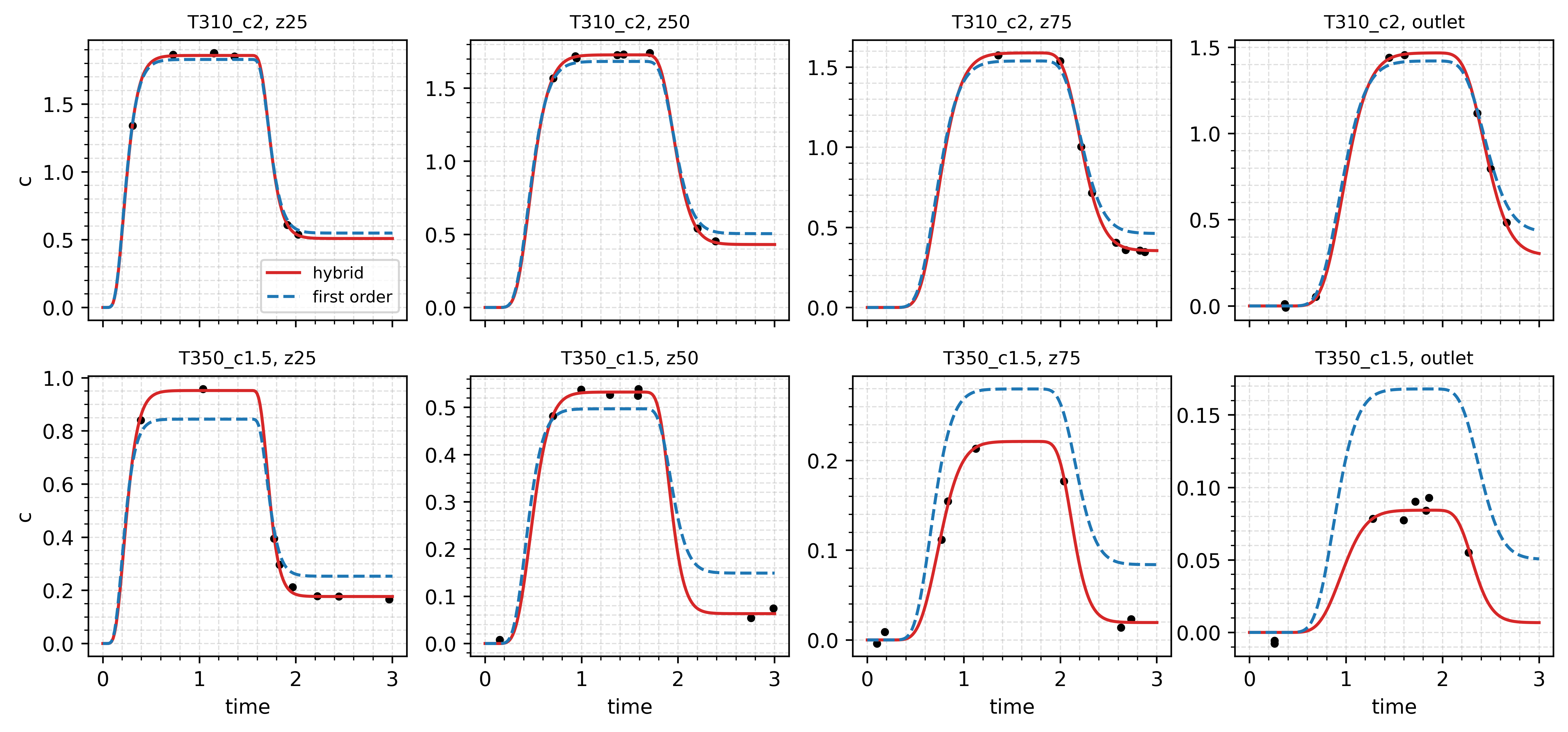
The first-order model also gets its constants wrong. It fits $E_a/R=5139$ K against a true 4000 K. The true effective coefficient is $k(T)/(1+Kc)$. Cold runs convert little, so $c$ stays high and the coefficient is suppressed by the denominator; hot runs consume the reactant, so $c$ is low and the coefficient is close to $k(T)$. Seen through a first-order model, the rate rises with temperature faster than Arrhenius alone, and the fit reads that as a larger activation energy.

The learned rate law matches the truth across the measured box:

$c$	$T$ (K)	true $r$	learned $r$
0.2	310	0.196	0.196
1.5	310	0.515	0.524
0.2	350	0.857	0.840
1.5	350	2.249	2.264

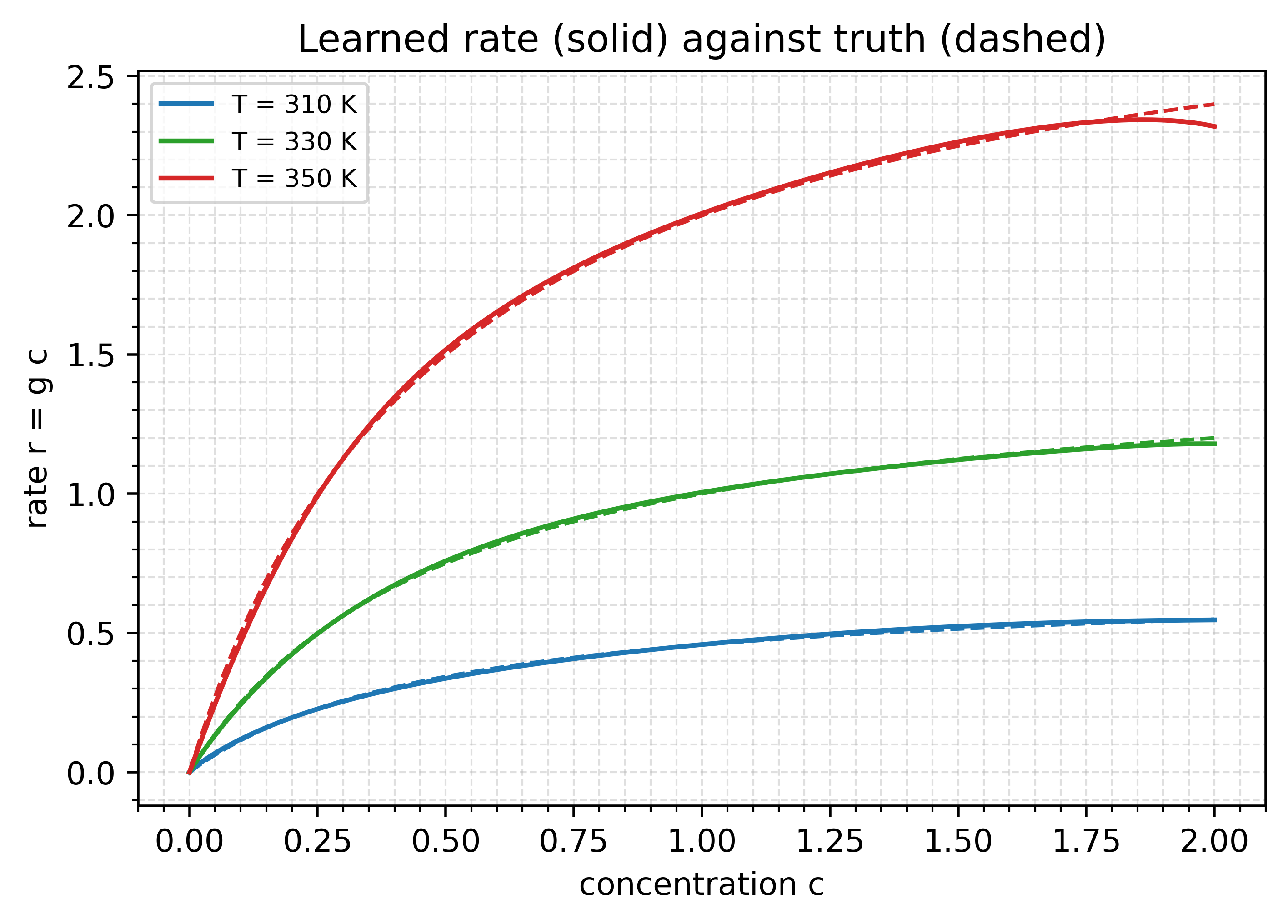
At 350 K the learned curve bends away from the truth above $c\approx 1.8$. No hot experiment reaches that concentration, since the hottest feed is 1.5 and the reaction is fast. The network has no data there.

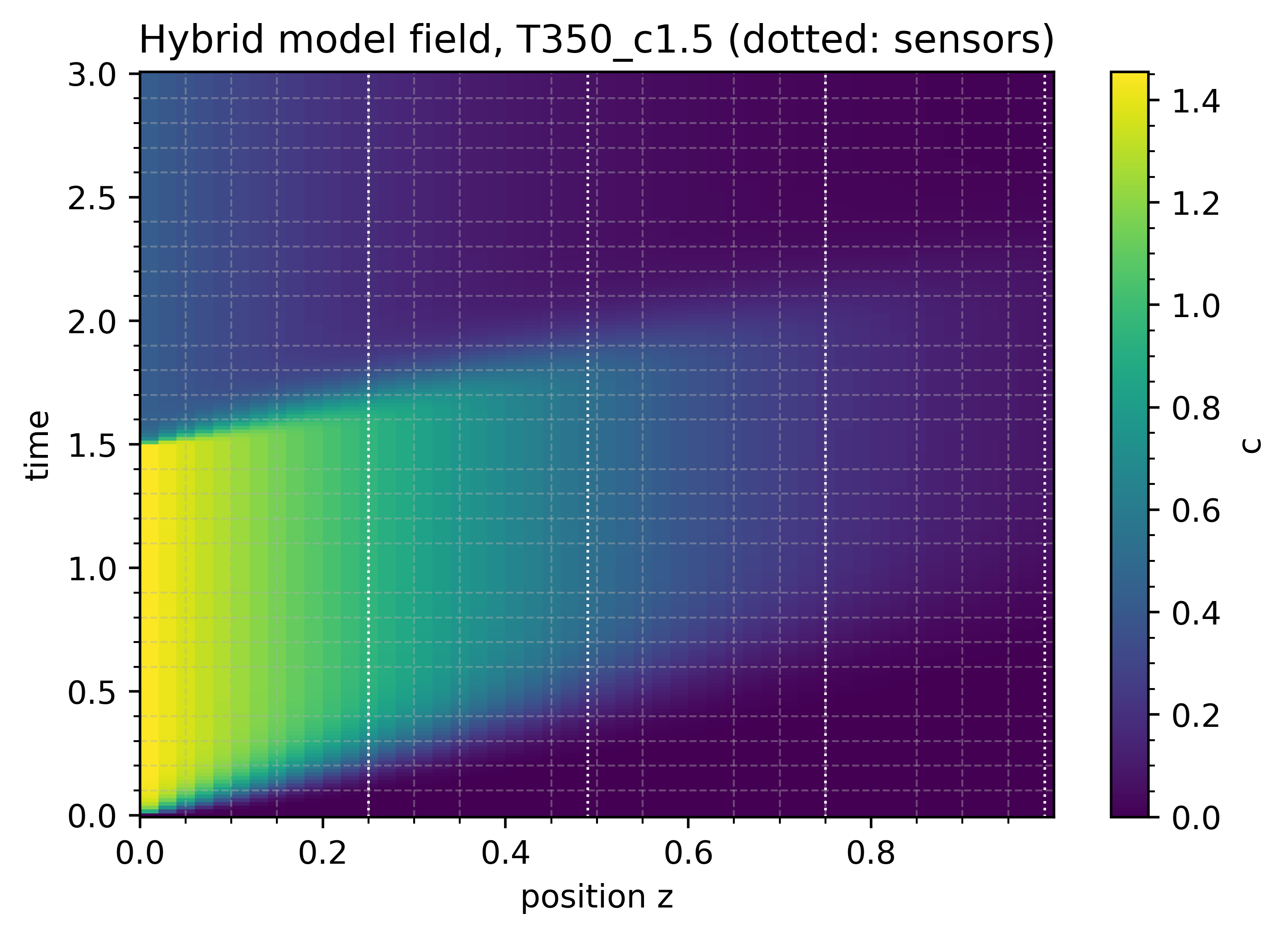
The full field of the hottest run shows what the sensors sample: the start-up front, the feed drop at $t=1.5$, and conversion along the tube.

Things to try

• Change N_CELLS to 200 and time a run with diffrax.Tsit5() against diffrax.Kvaerno3().
• Keep only the outlet in SENSORS and compare the recovered rate law. One channel sees the integrated effect of the whole tube.
• Replace RecursiveCheckpointAdjoint with diffrax.DirectAdjoint() and compare compile time and memory.
• Add a hot experiment with feed 2.0 to CONDITIONS and check that the learned curve at 350 K follows the truth to $c=2$.