Shapley effects

Sobol indices stop adding up when you care about interactions. S1 sums to less than 1, because the variance an interaction creates belongs to no single input. ST sums to more than 1, because it hands that same variance to every participant in full. Neither is a budget you can divide.

Shapley effects are the fix. You finish this page with one number per input, the numbers sum to 1, and you have the diagnostic that says whether they are worth reporting.

What gets distributed, and why it sums

Fit a surrogate and you get a partial variance $V_{u}$ for every subset $u$ of inputs the surrogate models. $V_{{1}}$ is what x1 does alone. $V_{{1, 3}}$ is the extra variance the x1-x3 pair creates that neither creates alone. The Shapley effect of input $i$ splits each subset's variance evenly among its members (Owen, 2014; Song, Nelson & Staum, 2016):

S h_{i} = \sum_{u : i \in u} \frac{V_{u}}{| u |}

Sum that over all $i$ . Each subset $u$ is counted once for each of its $| u |$ members, at $V_{u} / | u |$ apiece, so it contributes exactly $V_{u}$ . The total is $\sum_{u} V_{u}$ , the whole decomposed variance. Divide through by it and the effects sum to 1 by construction, not by luck.

That construction is also the warning. The sum is 1 whatever the surrogate did, including nothing useful, because it is a share of what the surrogate captured. Fit quality lives in a separate field, explained_variance, and the last section of this page is about reading it.

jaxgsa computes the allocation from a fitted surrogate's variance decomposition, so there is no permutation Monte Carlo and no extra model runs. S1 and ST come off the same fit, which makes the bracketing S1 <= Sh <= ST directly checkable.

Reach for Shapley effects when you need a single ranked importance score that divides a fixed budget, or when interactions matter and you refuse both to drop them (S1) and to double-count them (ST). Your inputs must be independent; the caveats section covers what to do when they are not.

The full script is examples/shapley_gsa.py, run with uv run python examples/shapley_gsa.py.

Import style

There is a standalone entry point, and a method on any fitted PCE or HDMR result:

python

import jaxgsa
# jaxgsa.shapley.analyze(problem, X, Y)   # fits, then allocates
# jaxgsa.pce.analyze(...).shapley()       # allocate from a fit you already have
# jaxgsa.hdmr.analyze(...).shapley()

Use shapley.analyze when Shapley effects are what you came for. Use .shapley() when you already have a fit and want the allocation for free.

Scalar example (Ishigami)

Ishigami is a three-input benchmark that ships with jaxgsa. Any (X, Y) pairs work, so plain Monte Carlo samples are enough. order=8 is the argument that matters. Ishigami's sine terms need a degree-8 polynomial, and the default order=3 under-fits badly enough to trip the warning shown later.

python

import jax.numpy as jnp
import jaxgsa
from jaxgsa.benchmarks.ishigami import PROBLEM, evaluate

X = jnp.asarray(jaxgsa.sampling.monte_carlo(PROBLEM, n=2000, seed=42))
Y = evaluate(X)

result = jaxgsa.shapley.analyze(PROBLEM, X, Y, order=8)

print("Sh:", result.Sh)
print("sum:", result.Sh.sum())
print("S1:", result.S1)
print("ST:", result.ST)
print("explained_variance:", result.explained_variance)

text

jaxgsa.shapley.analyze
  problem: D=3 (x1, x2, x3)
    marginals: uniform=3
    correlation: independent
    output: N=2000 runs, T=1 x K=1 output slice
    invalid: none found in 2000 rows (policy 'raise')
  timing:
    backend fit + Shapley (includes compile on the first call): 2.112 s
    backend: pce
    order: 8
  results: top 3 of 3 parameters by Sh
    1. x2  Sh=0.4418
    2. x1  Sh=0.4362
    3. x3  Sh=0.122
Sh: [0.43615592 0.44182348 0.12202042]
sum: 0.9999998
S1: [3.1413424e-01 4.4180435e-01 9.9179010e-07]
ST: [0.55818665 0.4418516  0.24404898]
explained_variance: 1.0339365

The summary block prints by default in 1.0. verbose=False silences it. The backend: pce line is worth a glance, because it is the default and the rest of the page depends on which one ran.

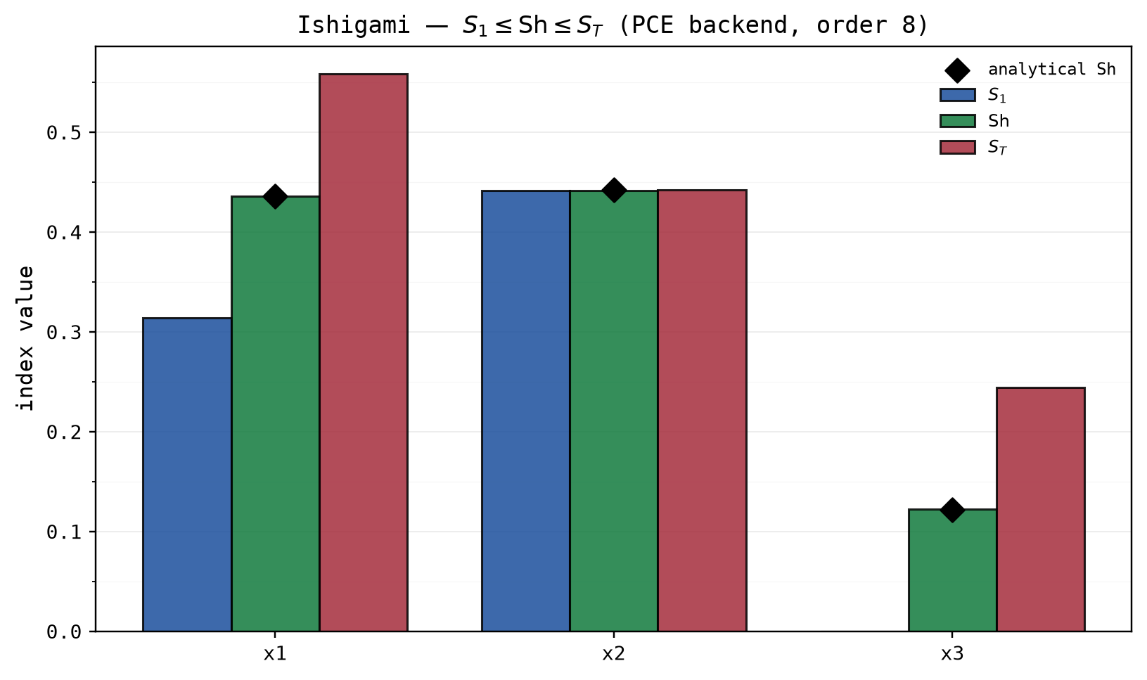
x3 is the whole argument for this method. Its first-order index is 9.9e-07, which is zero. x3 does nothing on its own. Its Shapley effect is 0.122, because it owns half of the x1-x3 interaction. Rank by S1 and you drop x3 from the model. Rank by ST and x3 scores 0.244, the full interaction, as does x1 for the same variance counted twice. The Shapley split of 0.122 each is the honest answer.

Ishigami has exactly one two-way interaction, so Sh = (S1 + ST) / 2 holds here and you can check it by hand: (0.31413 + 0.55819) / 2 = 0.43616.

x2 is the purely additive input on Ishigami — it enters only through 7 * sin(x2)^2 — so all three indices coincide for it: S1 = 0.4418, Sh = 0.4418 and ST = 0.4419 here, against an exact 0.4424. Where the three indices agree, the input acts alone and any one of them is the whole story.

The sum prints 0.9999998 rather than 1. That is float32 rounding over a 165-term expansion, not a modelling gap. Do not chase it.

Shapley effects on Ishigami bracketed between S1 and ST for every input, from the PCE backend

Ground-truth check

Ishigami, the linear model and Sobol-G ship analytical Shapley effects, so you can check against truth rather than against another implementation:

python

import numpy as np
from jaxgsa.benchmarks import ishigami

print("estimated: ", np.round(result.Sh, 4))
print("analytical:", np.round(ishigami.ANALYTICAL_SHAPLEY, 4))

text

estimated:  [0.4362     0.4418     0.12199999]
analytical: [0.4357 0.4424 0.1218]

Three decimals on all three inputs, worst gap 0.0006 on x2. Same ranking.

The script's own check is the same comparison as asserts, so it fails loudly instead of printing:

python

import numpy as np
from jaxgsa.benchmarks import ishigami

sh = np.asarray(result.Sh)
assert np.isclose(sh.sum(), 1.0, atol=1e-4)
print(f"sum(Sh) = {sh.sum():.6f}   (Shapley efficiency: exactly 1)")
print(f"max |error| = {np.max(np.abs(sh - ishigami.ANALYTICAL_SHAPLEY)):.4f}")

text

sum(Sh) = 1.000000   (Shapley efficiency: exactly 1)
max |error| = 0.0006

What it costs

Very little, and that is the point. The allocation is one matrix product against a boolean membership matrix of shape (n_terms, D). On the fit above, 165 terms and 3 inputs on an Apple M1 Pro, .shapley() takes 0.37 ms against 12.5 ms to redo the PCE fit. It costs zero model evaluations.

Compare that with the permutation Monte Carlo estimator, which walks random orderings of the inputs and needs a fresh batch of model runs at each step. Reading the effects off a surrogate replaces those runs with a fit you were going to do anyway. The bill you actually pay is the fit, and the fit is shared with S1 and ST.

Order as a convergence knob

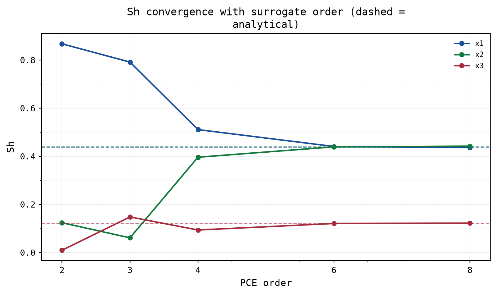
order is the surrogate's polynomial degree, and it is the knob you turn to make the allocation trustworthy. Sweep it on the same (X, Y) pair — no new model runs — and watch explained_variance approach 1 while the error against the analytical effects shrinks:

python

import numpy as np
from jaxgsa.benchmarks import ishigami

for order in (2, 3, 4, 6, 8):
    r = jaxgsa.pce.analyze(PROBLEM, X, Y, order=order).shapley()
    err = float(np.max(np.abs(np.asarray(r.Sh) - ishigami.ANALYTICAL_SHAPLEY)))
    print(f"order={order}  explained_variance={float(r.explained_variance):.3f}"
          f"  max |Sh - analytical| = {err:.4f}")

text

order=2  explained_variance=0.242  max |Sh - analytical| = 0.4315
order=3  explained_variance=0.476  max |Sh - analytical| = 0.3815
order=4  explained_variance=0.745  max |Sh - analytical| = 0.0749
order=6  explained_variance=0.983  max |Sh - analytical| = 0.0047
order=8  explained_variance=1.000  max |Sh - analytical| = 0.0006

Two things to notice. Even order=2 still sums to 1 — the efficiency normalization guarantees it — but it captured 24% of Var(Y), so its shares describe a truncated surrogate, not the model. order=3 under-fits here too, at explained_variance = 0.476, which is why the default order trips the below-0.5 warning on this benchmark. The allocation is only as good as the fit: order=8 reproduces the analytical effects to 0.0006. Each result also reports the order it actually fit as result.order (effective order: 8 in the scalar run above), so a saved analysis records its own truncation.

Shapley effect estimates converging onto the analytical values as the surrogate order is swept from 2 to 8

Backends

backend picks the surrogate that supplies the partial variances. The default is "pce".

backend="pce" reads subset variances off orthonormal polynomial coefficients (Sudret, 2008), exact within the fitted polynomial. Its knobs are order (default 3), ridge and fit_ratio. It refuses a declared problem.correlation.

backend="hdmr" fits the RS-HDMR B-spline surrogate and allocates its structural ANCOVA variances, truncated at maxorder. Its knobs are maxorder (default 2), m, maxiter, lambdax and slice_chunk_size. It accepts a declared correlation with include_correlative=True.

Both take (N,), (N, K) and (N, T, K) outputs as of 1.0. Older docs saying the PCE backend is scalar-only are wrong.

Backend knobs are not shared. Passing maxorder=3 with backend="pce" raises TypeError: analyze() got an unexpected keyword argument 'maxorder' rather than being ignored, so a typo cannot quietly change nothing.

Pick PCE for smooth responses, where it is exact and cheap. Pick HDMR for responses with kinks or plateaus, and for correlated inputs, which PCE refuses.

v1 limitation: both backends assume independent inputs for the allocation. The caveats below say what each one does if you declare a correlation anyway.

Multi-output example (HDMR backend)

N is samples, D inputs, K outputs, T timepoints. (N, K) gives indices of shape (K, D), and every output row sums to 1 on its own. (N, T, K) gives (T, K, D).

This example adds a second output with a known answer. Y2 is a sum of squares over symmetric bounds, so it has no interactions and its three inputs are interchangeable. Its shares must come out at 1/3 each, which is how you check the multi-output path did not scramble an axis. m=4 widens the B-spline basis, for the reason on the RS-HDMR page.

python

import jax.numpy as jnp
import jaxgsa
from jaxgsa.benchmarks.ishigami import PROBLEM, evaluate

X = jnp.asarray(jaxgsa.sampling.monte_carlo(PROBLEM, n=2000, seed=42))
Y1 = evaluate(X)
Y2 = jnp.sum(X**2, axis=1)
Y_multi = jnp.column_stack([Y1, Y2])

result = jaxgsa.shapley.analyze(PROBLEM, X, Y_multi, backend="hdmr", m=4)

print("Sh:", result.Sh)
print("row sums:", result.Sh.sum(axis=-1))
print("explained_variance:", result.explained_variance)

text

jaxgsa.shapley.analyze
  problem: D=3 (x1, x2, x3)
    marginals: uniform=3
    correlation: independent
    output: N=2000 runs, T=1 x K=2 output slices
    invalid: none found in 2000 rows (policy 'raise')
  timing:
    backend fit + Shapley (includes compile on the first call): 2.266 s
    backend: hdmr
    order: 2
  results: top 3 of 3 parameters by Sh, mean over 2 output slices
    1. x2  Sh=0.3943
    2. x1  Sh=0.3734
    3. x3  Sh=0.2323
Sh: [[0.4217161  0.45171946 0.12656444]
 [0.32505286 0.3369298  0.33801743]]
row sums: [1.        1.0000001]
explained_variance: [1.0094421 0.9541204]

Row 1 is Ishigami and reproduces the scalar answer to two decimals. Row 2 is the sum of squares and comes out [0.325, 0.337, 0.338], within 0.01 of the 1/3 the construction demands. The residual spread is finite-sample noise in a 2000-row fit.

The results: table averages over output slices, which is fine for a quick glance and useless when the outputs disagree. Read result.Sh per row. explained_variance also has one entry per output, so a bad fit on one output cannot hide behind a good fit on the other.

The `explained_variance` diagnostic

Sh is normalized by the surrogate's total decomposed variance $\sum_{u} V_{u}$ , so it sums to 1 however badly the surrogate fits. Fit quality is reported separately:

explained_variance = \frac{\sum_{u} V_{u}}{Var (Y)}

Near 1 is a faithful surrogate. Below 1 means truncation or fit error left variance unexplained. Above 1 means an overfit surrogate over-counted shared variance. A JaxgsaWarning fires below 0.5 or above 1.3.

Here is what a bad fit looks like. Same data, order=2:

python

low = jaxgsa.pce.analyze(PROBLEM, X, Y1, order=2, verbose=False).shapley()
print("Sh:", low.Sh)
print("sum:", low.Sh.sum())
print("explained_variance:", low.explained_variance)

text

JaxgsaWarning: jaxgsa.shapley: surrogate explained_variance is below 0.5;
Shapley effects may be unreliable
Sh: [0.86724067 0.12359249 0.0091669 ]
sum: 1.0000001
explained_variance: 0.24137108

The sum is still 1. The effects are still ordered, positive, and completely wrong: x1 gets 0.867 against its true 0.436, x2 collapses from 0.442 to 0.124, and x3 all but vanishes. A degree-2 polynomial captured 24% of Ishigami's variance, and these are honest shares of that 24%.

The sum tells you nothing about fit quality. Only explained_variance does. Read it first, every time. If it is off, raise order or maxorder and refit until it settles near 1.

One consequence of the normalization. With backend="pce" the S1 and ST on the result match jaxgsa.pce.analyze exactly. With backend="hdmr" they differ from jaxgsa.hdmr.analyze's by a factor of explained_variance, because HDMR normalizes by Var(Y) instead.

xarray export

to_dataset() returns a labeled xarray.Dataset, so you select an input or an output by name:

python

ds = result.to_dataset()
print(ds)
print(ds.Sh.sel(param="x1").values)

text

<xarray.Dataset> Size: 120B
Dimensions:             (output: 2, param: 3)
Coordinates:
  * output              (output) <U2 16B 'y0' 'y1'
  * param               (param) <U2 24B 'x1' 'x2' 'x3'
Data variables:
    Sh                  (output, param) float32 24B 0.4217 0.4517 ... 0.338
    S1                  (output, param) float32 24B 0.3006 0.4445 ... 0.338
    ST                  (output, param) float32 24B 0.5428 0.4589 ... 0.338
    explained_variance  (output) float32 8B 1.009 0.9541
Attributes:
    backend:              hdmr
    order:                2
    include_correlative:  False
[0.4217161  0.32505286]

ds.Sh.sel(param="x1") gives x1's share for each output. explained_variance carries no param dimension, so it prints one value per output. The attributes record which backend and truncation produced the numbers, which matters when the dataset outlives the session. Set problem.output_names to replace y0 and y1 with real names, and pass time_coords to label a time dimension.

Shape rules

Y shape	backend	Sh / S1 / ST shape	explained_variance
`(N,)`	pce or hdmr	`(D,)`	`()`
`(N, K)`	pce or hdmr	`(K, D)`	`(K,)`
`(N, T, K)`	pce or hdmr	`(T, K, D)`	`(T, K)`

D is always the last axis. Without problem.output_names, a 2D Y is read as (N, K). With exactly one entry in output_names it is read as (N, T), timepoints of that single output, and flows through as (N, T, 1). A pre-reshaped (N, T, 1) array works too.

Practical caveats

Independent inputs are assumed, and the PCE backend enforces it. Pass a problem with a declared correlation and shapley.analyze raises ValueError rather than returning a silently wrong allocation. The message names the alternatives.

The HDMR route under dependence is an approximation, not a Shapley effect.backend="hdmr" with include_correlative=True allocates the total ANCOVA contribution Sa + Sb and does accept a declared correlation. It is an ANCOVA-based attribution. A true conditional-variance Shapley effect needs an estimator of the variance remaining once a group of inputs is held fixed, and jaxgsa does not have one yet. For conditional-variance indices under dependence, leave Shapley behind: VKOGA works from given data through a kernel surrogate, Kucherenko uses its own design and your actual model. Neither returns a per-parameter allocation summing to 1.

Interactions past the truncation are simply absent. Anything beyond order for PCE or maxorder for HDMR contributes nothing to the allocation, and explained_variance is the only place that absence shows up.

The HDMR backend inherits jaxgsa.hdmr.analyze's contract: at least 300 samples, maxorder in {1, 2, 3}, clamped with a warning when D < maxorder.

Shapley effects ​

What gets distributed, and why it sums ​

Import style ​

Scalar example (Ishigami) ​

Ground-truth check ​

What it costs ​

Order as a convergence knob ​

Backends ​

Multi-output example (HDMR backend) ​

The explained_variance diagnostic ​

xarray export ​

Shape rules ​

Practical caveats ​

See also ​

Shapley effects

What gets distributed, and why it sums

Import style

Scalar example (Ishigami)

Ground-truth check

What it costs

Order as a convergence knob

Backends

Multi-output example (HDMR backend)

The `explained_variance` diagnostic

xarray export

Shape rules

Practical caveats

See also