Comparing Methods on Ishigami
Different sensitivity methods answer different questions. This example runs eight methods on the same three-input model so you can see what each result means, then compare model evaluations and accuracy where the quantities are comparable.
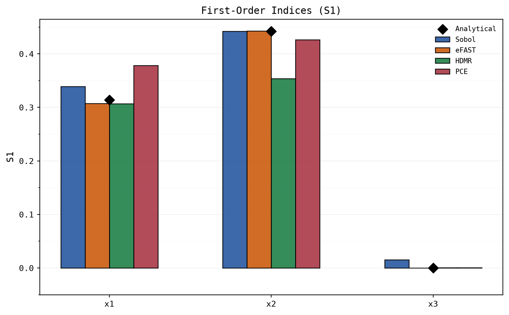
The Ishigami function has a useful surprise: its third input has almost no effect on its own, but matters through an interaction with the first input. Its analytical first-order indices are
The full script is examples/method_comparison.py, run with uv run examples/method_comparison.py.
The script prints the numbers below. Its wall times come from one machine and depend on hardware and JAX compilation. Use them only as a rough indication of cost.
Start with the question
| Question | Methods in this example | What to read |
|---|---|---|
| Which inputs explain output variation, alone and with interactions? | Sobol, eFAST, HDMR, PCE | S1 and ST |
| Which inputs can I rule out cheaply? | Morris, DGSM | Screening measure or bound, not a variance share |
| How should variation be shared among inputs, including interactions? | Shapley | Shapley effects |
| Which inputs change the whole output distribution? | Borgonovo delta | Delta measure |
Start with Sobol if you need both first and total effects and possibly pairwise interactions. Try Morris if you need to narrow many inputs before paying for a more detailed analysis. If you already have input and output samples, methods such as HDMR and PCE can use them directly. The method guide covers the remaining choices and assumptions.
What the comparison shows
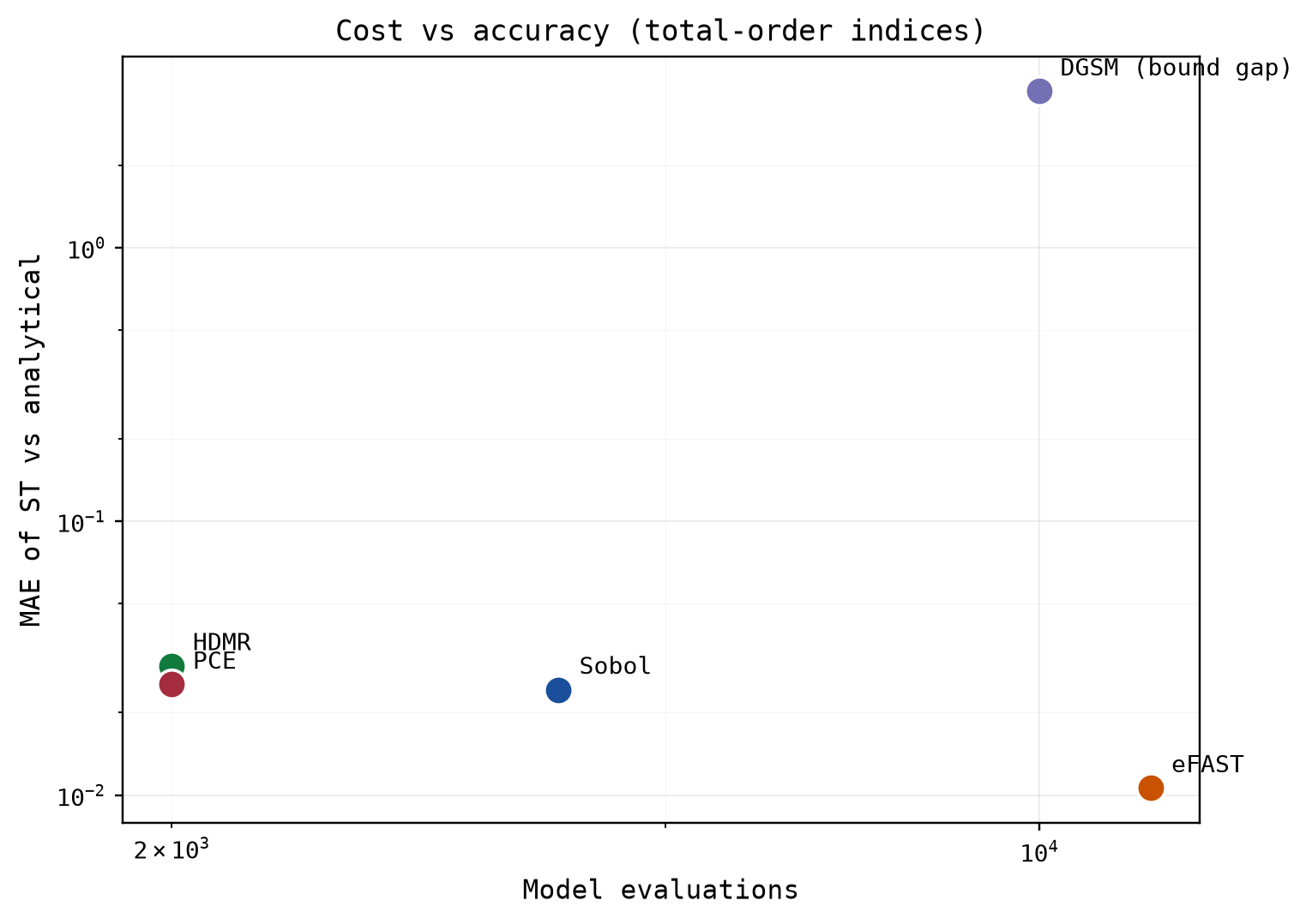
For methods that estimate S1 or ST, the table reports mean absolute error (MAE) against the analytical values above. Smaller is closer for this run. N evals counts model evaluations. A dash means that the method does not produce a comparable estimate.
| Method | S1 MAE | ST MAE | N evals | Wall time (s) |
|---|---|---|---|---|
| Sobol | 0.0136 | 0.0243 | 4,096 | 1.14 |
| eFAST | 0.0021 | 0.0106 | 12,288 | 0.37 |
| HDMR | 0.0320 | 0.0296 | 2,000 | 2.14 |
| PCE | 0.0271 | 0.0254 | 2,000 | 1.46 |
| DGSM (bound gap) | — | 3.7270 | 10,000 | 0.71 |
| Morris (screening) | — | — | 64 | 0.56 |
| Shapley (Sh) | 0.0271 | 0.0254 | 2,000 | 0.23 |
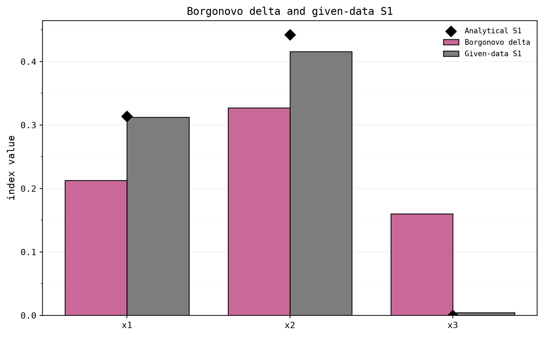
| Borgonovo delta | 0.0109 | — | 2,000 | 0.48 |
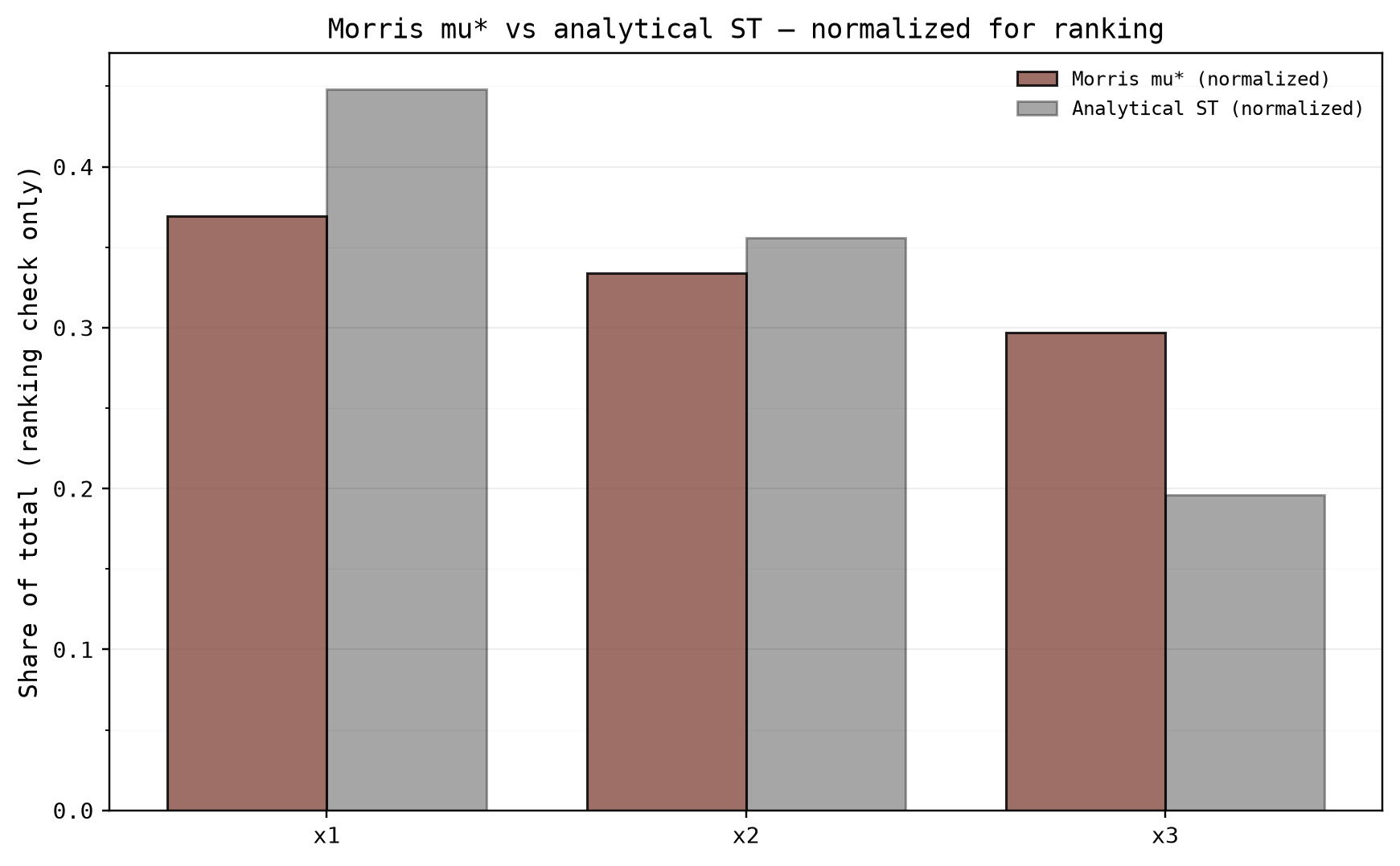
For this model and these sample sizes, eFAST's first-order estimates are closer to the analytical values than Sobol's, but use three times as many model evaluations. Sobol also gives pairwise interaction indices when its second-order option is enabled. Morris gives a screening ranking with only 64 evaluations; it does not estimate a share of output variance.
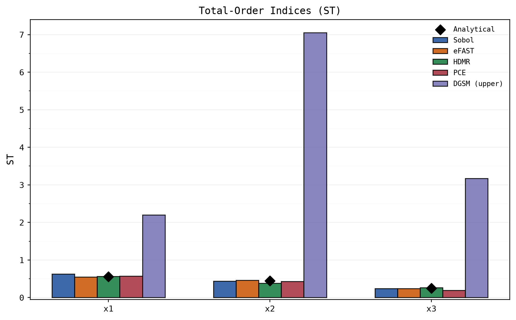
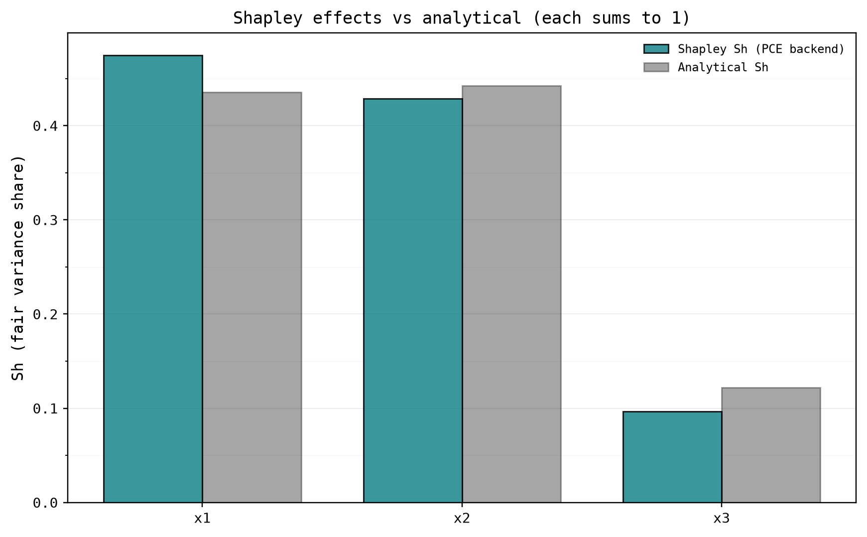
The DGSM row needs special care: 3.7270 is the error of its upper bound for ST, not an index estimate. The bound is loose for this non-monotone model, so use DGSM here to screen inputs rather than to estimate their total effects. Shapley and Borgonovo report S1 through their given-data estimators; the Shapley run uses the same PCE surrogate as the PCE row, explaining their matching S1 values.
The time columns also cover different work. Sobol, eFAST, and Morris include sampling, model evaluation, and analysis. HDMR, PCE, Shapley, and Borgonovo time analysis of shared precomputed samples. DGSM times analysis that evaluates the model internally with automatic differentiation. Do not compare the wall times as if all rows included the same steps.
HSIC and PAWN are given-data methods outside this comparison. They measure dependence or changes in the output distribution. See Choosing a method for the full method comparison and assumptions behind each choice.
Figures
The script draws six figures; the four index charts are grouped bars against the analytical values (black diamonds), Morris is a normalized ranking check, and the last chart is the cost-vs-accuracy trade-off.