Non-Uniform Inputs

A marginal is the distribution of one input on its own. Sobol indices are defined against those marginals, so declaring the wrong one does not give you a slightly noisier answer. It gives you the right answer to a question about a system you do not have. The second half of this page shows one such mistake reversing an importance ranking end to end.

jaxgsa.Problem.from_dict(...) takes the (low, high) uniform shorthand and tagged specs for Gaussian and truncated Gaussian inputs. A truncated Gaussian is a Gaussian restricted to an interval, with the remaining probability rescaled to sum to one.

The full script is examples/oakley_ohagan_15d.py, run with uv run python examples/oakley_ohagan_15d.py.

Declare a mixed problem

One input of each kind. The key becomes the parameter name, and dist marks the entry as a distribution spec rather than a bounds pair.

import jax.numpy as jnp
import numpy as np
from scipy.stats import truncnorm

import jaxgsa

problem = jaxgsa.Problem.from_dict(
    {
        "uniform": (0.0, 2.0),
        "gaussian": {"dist": "gaussian", "mean": 1.0, "variance": 2.25},
        "truncated": {
            "dist": "gaussian",
            "mean": 0.5,
            "variance": 1.44,
            "low": -3.1,
            "high": 4.1,
        },
    }
)

The truncation sits at 3 standard deviations either side of the mean, because $0.5\pm 3\times 1.2$ is $[-3.1,4.1]$. Hold on to that. It is the number the last section abuses.

Rules for Gaussian specs:

• mean and variance describe the parent Gaussian, before truncation.
• low and high are optional and independent. Truncating one side only is fine.
• When either bound is present, jaxgsa.sobol.sample() uses a true truncated normal transform. It does not clip samples that fall outside.
• An unbounded Gaussian is still bounded in practice, at $\pm 7.0345$ standard deviations. Inverse-CDF sampling has to keep the unit coordinate off 0 and 1, and that clip is what the distance works out to.
• Problem.from_dict(params, truncate_gaussians=q) fills low and high into every Gaussian that does not already declare them, at that marginal's own q and 1 - q quantiles. Sides you wrote yourself are left alone. Use it when one bounded input model has to be shared across methods.

Check against a closed form

Use a linear model here, because its Sobol indices are known exactly. That turns the run into a test of the sampler rather than a demonstration of it. For

$$y=\sum _i{a}_i{x}_i$$

the first-order and total-order indices are the same number,

$$S_i=\frac{a_i^2\mathrm{Var}(X_i)}{\sum _j{a}_j^2\mathrm{Var}(X_j)}$$

because a sum of separate terms has no interactions for ST to pick up.

coeffs = jnp.array([1.5, -0.75, 0.7])

design = jaxgsa.sobol.sample(problem, n_samples=8192, calc_second_order=False, seed=101)
X = jnp.asarray(design.samples)
Y = X @ coeffs

result = jaxgsa.sobol.analyze(design, Y)

jaxgsa.sobol.sample: D=3, mode=first/total-order, base_n=2048, requested_runs>=8192, n_runs=10240, n_expanded=10240, duplicates_removed=0 (0.0%), scramble=True
jaxgsa.sobol.analyze
  problem: D=3 (uniform, gaussian, truncated)
    marginals: uniform=1, gaussian=2
    correlation: independent
    output: N=10240 runs, T=1 x K=1 output slice
    invalid: none found in 2048 Saltelli groups (policy 'raise')
  timing:
    estimators (includes compile on the first call): 0.3932 s
    slice_chunk_size: 1 (resolved from the memory budget)
    estimator: saltelli-jansen
  results: top 3 of 3 parameters by ST
    1. gaussian   ST=0.4681
    2. uniform    ST=0.2777
    3. truncated  ST=0.2544

Read marginals: uniform=1, gaussian=2 first. Two Gaussians, because a truncated Gaussian is counted as a Gaussian. If that line says uniform=3 you have made the mistake this page is about, and you can catch it before the analysis finishes.

The exact answer needs each input's variance. The uniform gives $(\text{high}-\text{low}{)}^2/12$, the Gaussian gives the declared 2.25, and scipy.stats.truncnorm gives the truncated one. Its a and b arguments are the bounds measured in standard deviations from the mean, which is not the same convention as low and high.

std = np.sqrt(1.44)
a, b = (-3.1 - 0.5) / std, (4.1 - 0.5) / std

variances = np.array([(2.0 - 0.0) ** 2 / 12.0, 2.25, truncnorm.var(a, b, loc=0.5, scale=std)])
weights = np.square(np.asarray(coeffs)) * variances
analytical = weights / weights.sum()

np.set_printoptions(precision=4, suppress=True)
print("S1        ", np.asarray(result.S1))
print("ST        ", np.asarray(result.ST))
print("analytical", analytical)

S1         [0.2778 0.4679 0.2543]
ST         [0.2777 0.4681 0.2544]
analytical [0.2775 0.4683 0.2541]

Every entry agrees with the closed form to within 0.0004, and S1 agrees with ST to within 0.0002. Both facts are checks, not results. The first says the truncated normal transform is drawing from the distribution you declared. The second says the estimator found no interaction in a model that has none, so what you are seeing is the noise floor at base_n=2048, and it is about $2\times {10}^{-4}$. Any interaction smaller than that in a real model would be invisible here.

result.S2 is None, because calc_second_order=False never built the design rows it needs. The output was one number per run, so result.S1 has shape (D,). See Multi-Output & Time-Series for what happens to that shape when the model returns more.

Getting the marginal wrong flips the ranking

Here is the mistake, and it is a tempting one. You know truncated lives in $[-3.1,4.1]$. You do not have its distribution to hand. So you declare the range as a uniform and move on.

wrong = jaxgsa.Problem.from_dict(
    {
        "uniform": (0.0, 2.0),
        "gaussian": {"dist": "gaussian", "mean": 1.0, "variance": 2.25},
        "truncated": (-3.1, 4.1),
    }
)

design_w = jaxgsa.sobol.sample(wrong, n_samples=8192, calc_second_order=False, seed=101, verbose=False)
Xw = jnp.asarray(design_w.samples)
result_w = jaxgsa.sobol.analyze(design_w, Xw @ coeffs)

jaxgsa.sobol.analyze
  problem: D=3 (uniform, gaussian, truncated)
    marginals: uniform=2, gaussian=1
    correlation: independent
    output: N=10240 runs, T=1 x K=1 output slice
    invalid: none found in 2048 Saltelli groups (policy 'raise')
  timing:
    estimators (includes compile on the first call): 0.0007109 s
    slice_chunk_size: 1 (resolved from the memory budget)
    estimator: saltelli-jansen
  results: top 3 of 3 parameters by ST
    1. truncated  ST=0.5124
    2. gaussian   ST=0.306
    3. uniform    ST=0.1815

The timing line dropped from 0.3932 s to 0.0007 s, because the shapes are the same and XLA reuses the compiled kernels from the first analysis. Timings in a verbose block only mean something on the first call of a given shape.

truncated went from last at 0.2544 to first at 0.5124, and every other input moved down a place. The whole ranking reversed. Nothing about the model changed. The bounds are identical. Only the shape inside them changed.

The arithmetic is one line. The sampled variance of that column is 1.4014 under the truncated Gaussian and 4.32 under the uniform, because a uniform on a $6\sigma$ window has variance $(6\sigma {)}^2/12=3{\sigma }^2$. A first-order Sobol index for a linear model is proportional to input variance, so tripling the variance roughly triples the index. Check it yourself with np.var(np.asarray(X), axis=0) against np.var(np.asarray(Xw), axis=0).

Nothing in either run looks wrong. Both agree with their own closed form. Both report clean diagnostics. The wrong result is a correct sensitivity analysis of a system whose third input is uniform, and you do not have that system. This is why the failure is worth a section. It is silent, and the only place it shows is the one-line marginals: count in the verbose block.

The direction of the error is predictable. Substituting a uniform for a bell-shaped marginal on the same support always inflates the variance, so it always overstates that input. The factor is $3$ at $\pm 3\sigma$ and grows with the width of the window. A range you are confident about, combined with a shape you guessed, is the worst of both.

High-dimensional: Oakley & O'Hagan (15 inputs)

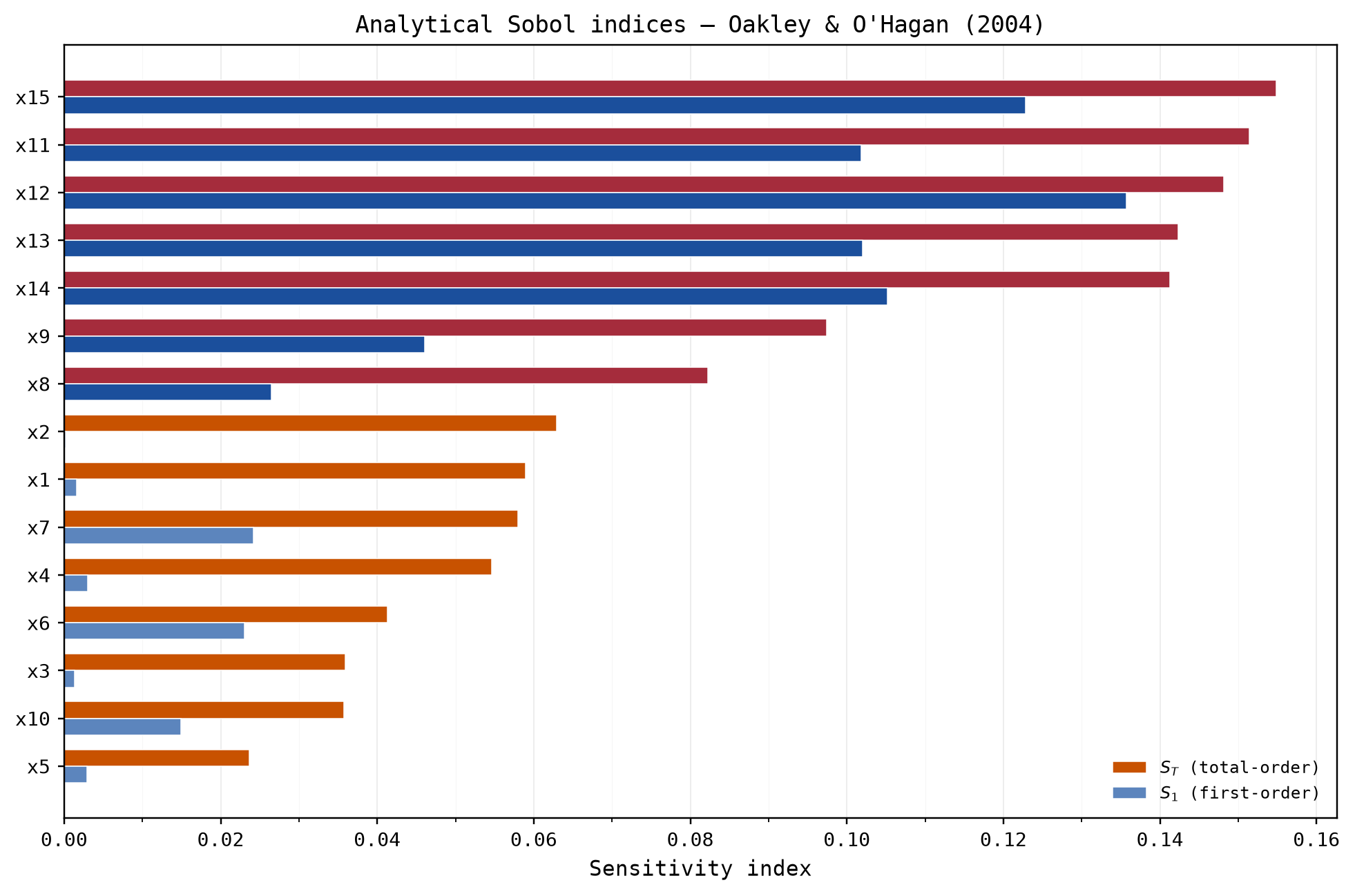
This section puts three methods on the 15-input Oakley & O'Hagan benchmark, where every marginal is N(0, 1) and all indices are known analytically. The published coefficients grow toward the higher indices, which makes the inputs an importance gradient in three tiers: x1-x5 nearly inert (analytical $S_1$ at or below 0.003), x6-x10 intermediate ($S_1$ between 0.015 and 0.046), x11-x15 dominant ($S_1$ between 0.10 and 0.136). The first-order indices sum to 0.7112; because that is below 1, the remaining variance lives in interactions, so each method below must get total-order indices right, not just main effects.

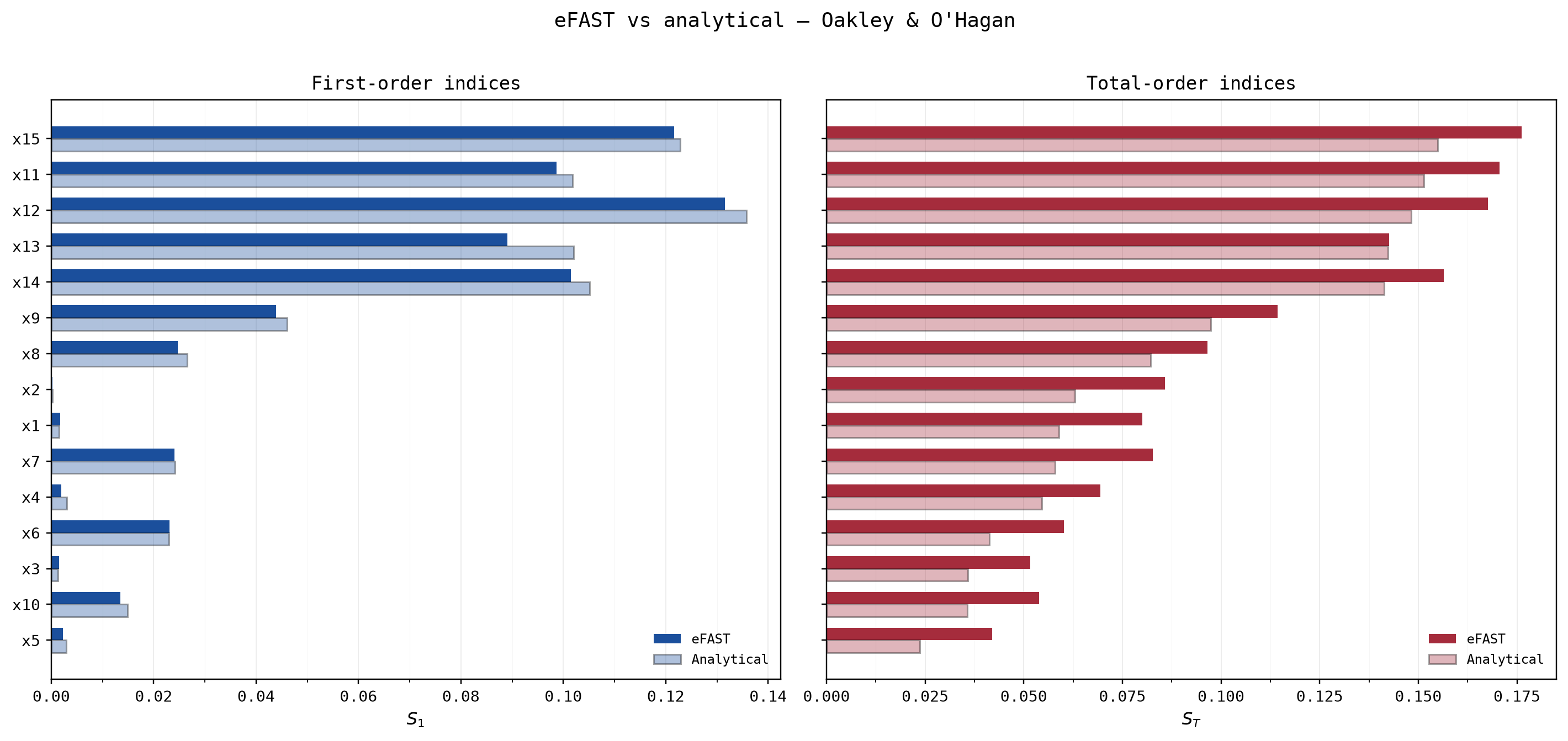
eFAST: Gaussian inputs through the inverse CDF. This is the first example on this page where eFAST handles a non-uniform marginal. sample() draws each search curve in uniform [0, 1] with Cukier's transform and maps those samples through the marginal CDFs into physical space; for this problem that mapping is the Gaussian inverse CDF. The 15 curves at 4096 points each cost 61440 model runs.

efast_samples = jaxgsa.efast.sample(problem, n_per_curve=4096, M=4, seed=42)
Y_ef = oakley_ohagan.evaluate(jnp.asarray(efast_samples.samples))

efast_result = jaxgsa.efast.analyze(efast_samples, Y_ef)
print(efast_result)

The top five by eFAST $S_T$ are x15 (0.1761), x11 (0.1706), x12 (0.1676), x14 (0.1565), x13 (0.1426): the x11-x15 block, with estimates a little above the analytical values (x15: 0.1761 vs 0.1549).

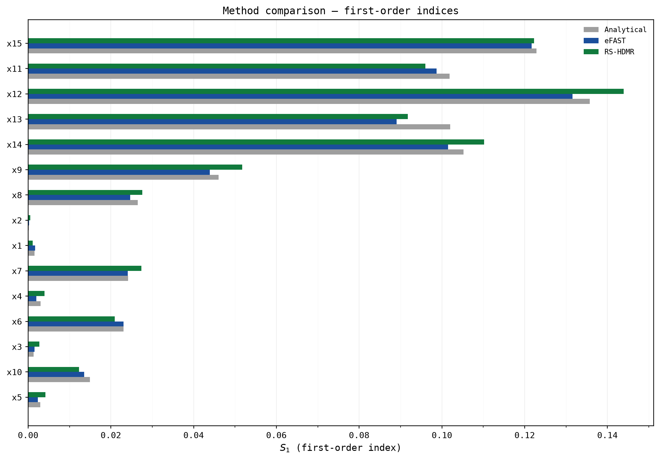
RS-HDMR: existing samples, no structured design. RS-HDMR works from plain i.i.d. draws: 3000 Gaussian samples, second-order component functions (maxorder=2), and m=2 basis functions per dimension.

key = jax.random.key(0)
X_hd = jax.random.normal(key, (3000, problem.num_vars))
Y_hd = oakley_ohagan.evaluate(jnp.asarray(X_hd))

hdmr_result = jaxgsa.hdmr.analyze(problem, X_hd, Y_hd, maxorder=2, m=2)
print(hdmr_result)

The script warns that the fitted terms overlap (S.sum() = 1.74), so the HDMR values run above the analytical ones (x14: 0.2466 vs 0.1413). Read them as a ranking, which is all the comparison below uses.

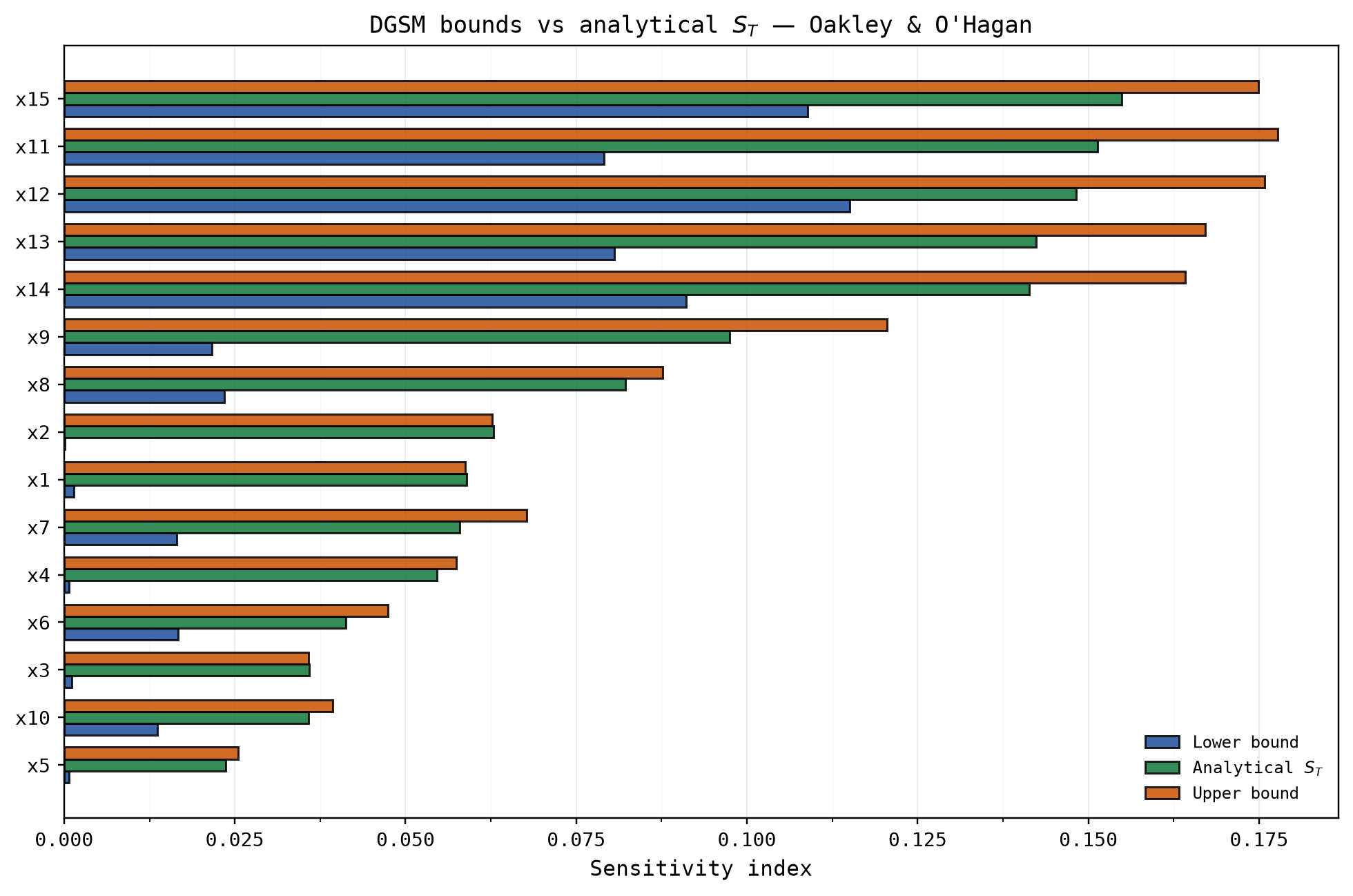
DGSM: one autodiff sweep. DGSM needs the unbatched wrapper, defined at its single use site. The script checks it on a zero row first: f(0) = 15.7560.

def oakley_fn(x):
    """Unbatched Oakley & O'Hagan: (15,) -> ()."""
    return oakley_ohagan.evaluate(x[None, :])[0]

X_dg = jaxgsa.sampling.monte_carlo(problem, n=10_000, seed=42)
dgsm_result = jaxgsa.dgsm.analyze(problem, oakley_fn, jnp.asarray(X_dg))
print(dgsm_result)

All 15 marginals are untruncated Gaussians, so here both bounds carry their proofs — Poincare above, Kucherenko-Song below — and the Poincare constant is the variance, 1, tighter than a uniform marginal of comparable width would give. The $\nu$ ranking (x11 10.75, x12 10.63, x15 10.58, x13 10.11, x14 9.929) already names the dominant block.

Top-5 ranking accuracy. The check asks each method for its five largest total-order inputs and counts how many match the analytical top five:

Method	Top-5 parameters	Match
Analytical	x11, x12, x13, x14, x15	--
eFAST ($S_T$)	x11, x12, x13, x14, x15	5/5
RS-HDMR ($S_T$)	x8, x11, x12, x14, x15	4/5
DGSM (upper bound)	x11, x12, x13, x14, x15	5/5

All three methods land the x11-x15 block. HDMR misses one slot: x13 drops out and x8 (analytical $S_T$ 0.0822) takes its place, consistent with the overlap warning above.

The method to pick depends on what you can still choose. Pick eFAST when you can choose a structured sampling budget: 61440 runs buy the full decomposition at 15 dimensions. Pick RS-HDMR when the dataset already exists as plain samples: 3000 draws found the block, with one ranking error. Pick DGSM when the model is differentiable: 10000 Monte Carlo rows and one autodiff sweep recover the exact top five.

Practical notes

• problem.bounds is None as soon as any Gaussian spec is present. That is the intended signal that the problem is no longer finite-bounds-only. Code that reaches for problem.bounds to build its own uniform sample raises on the None rather than returning a wrong answer.
• Save and load carries the marginals. The JSON metadata records the declared specs, so SobolSamples.load() rebuilds the same distributions rather than re-reading bounds.
• jaxgsa.hdmr.analyze() handles Gaussian and truncated Gaussian inputs by mapping through the CDF onto [0, 1] before it fits the surrogate.
• jaxgsa.pce.analyze() picks its polynomial family from how tight the truncation is. A narrow truncation is a different measure, so it goes through the truncated CDF and onto Legendre. A wide one, meaning every declared bound at least 5 standard deviations out, keeps Hermite, because forcing Legendre there makes the fit visibly worse. On Oakley-O'Hagan at order 3 the leave-one-out RMSE went from 0.93 to 1.70 and the largest S1 error from 0.0023 to 0.0054. The $\pm 3\sigma$ truncation declared on this page counts as narrow, so PCE would put it on Legendre. Above order 7 Legendre wins even for a wide truncation, because the Hermite Gram defect against a truncated measure grows with degree.

See also

• Basic Example for the smallest uniform-only run, and for how fast the estimator error falls with sample size.
• Correlated Inputs when the inputs are not independent, which the marginals alone cannot express.
• Save and Reload Samples to persist a mixed design.
• API Reference for the exact TypedDict shapes and the Problem.bounds contract.