eFAST (extended FAST)

eFAST gives you a first-order index S1 and a total-order index ST for every input. S1 is the share of output variance the input drives on its own. ST adds every interaction it takes part in. There is no S2, so eFAST will tell you that two inputs interact and never tell you which two.

The cost is n_per_curve * D model runs and nothing else. One curve per input, a fixed number of points on each, no replicates. That number is the whole budget, and you choose it before you evaluate anything.

The API is the same shape as the Sobol workflow: efast.sample(...) builds the design, efast.analyze(...) consumes it. Switching methods is a one-line change — swap the sample call and keep the rest.

The full script is examples/efast_gsa.py, run with uv run python examples/efast_gsa.py.

The frequency trick

Take one input, call it the focal input. Instead of drawing a random cloud, eFAST walks a single path through the input space and makes every input oscillate along it at its own integer frequency. The focal input gets the highest frequency, omega_0. The others get much lower ones.

Now Fourier-transform the output along that path. If the focal input drives the output, the output wobbles at omega_0 and at its harmonics 2*omega_0, 3*omega_0, and so on. Power sitting at those harmonics is the focal input's own contribution, and dividing it by the total power gives S1. Everything below omega_0 / 2 came from the other inputs, so one minus that share is ST.

One path per input, so D paths, and the model runs once per point on each.

Two knobs control the trick, and both of them can break it quietly.

• n_per_curve sets omega_0 = (n_per_curve - 1) // (2 * M). A longer curve buys a higher focal frequency and more room between the frequencies.
• M, the interference factor, is how many harmonics of omega_0 get credited to the focal input. It is also what keeps the other inputs' carriers away from those harmonics: the highest carrier the sampler will assign sits at omega_0 / (2 * M).

The failure mode is aliasing. If a non-focal input's carrier has a harmonic that lands on omega_0, its power is charged to the focal input, and you get a confident wrong number in [0, 1] with no warning attached. The sections below show it happening.

Import style

from jaxgsa import efast
# efast.sample(...)
# efast.analyze(...)

Scalar example (Ishigami)

Build the design, evaluate the model on every row in order, then hand the design object back to analyze. Pass the object, not the raw array: n_per_curve, M and the problem travel inside it, so the analyzer cannot look for the wrong frequency.

import jax.numpy as jnp
from jaxgsa import efast
from jaxgsa.benchmarks.ishigami import PROBLEM, evaluate, ANALYTICAL_S1, ANALYTICAL_ST

samples = efast.sample(PROBLEM, n_per_curve=4096, M=4, seed=42)
print("shape:", samples.samples.shape, "n_runs:", samples.n_runs)

Y = evaluate(jnp.asarray(samples.samples))
result = efast.analyze(samples, Y)

print("S1:", result.S1)
print("ST:", result.ST)
print("exact S1:", ANALYTICAL_S1)
print("exact ST:", ANALYTICAL_ST)

jaxgsa.efast.sample: D=3, n_curves=3, n_per_curve=4096, n_runs=12288, M=4, omega_0=511
shape: (12288, 3) n_runs: 12288
jaxgsa.efast.analyze
  problem: D=3 (x1, x2, x3)
    marginals: uniform=3
    correlation: independent
    output: N=12288 runs, T=1 x K=1 output slice
    invalid: none found in 3 search curves (policy 'raise')
  timing:
    estimator (includes compile on the first call): 0.1799 s
    slice_chunk_size: auto (resolved from the memory budget)
    omega_0: 511, M: 4
  results: top 3 of 3 parameters by ST
    1. x1  ST=0.5507
    2. x2  ST=0.463
    3. x3  ST=0.2393
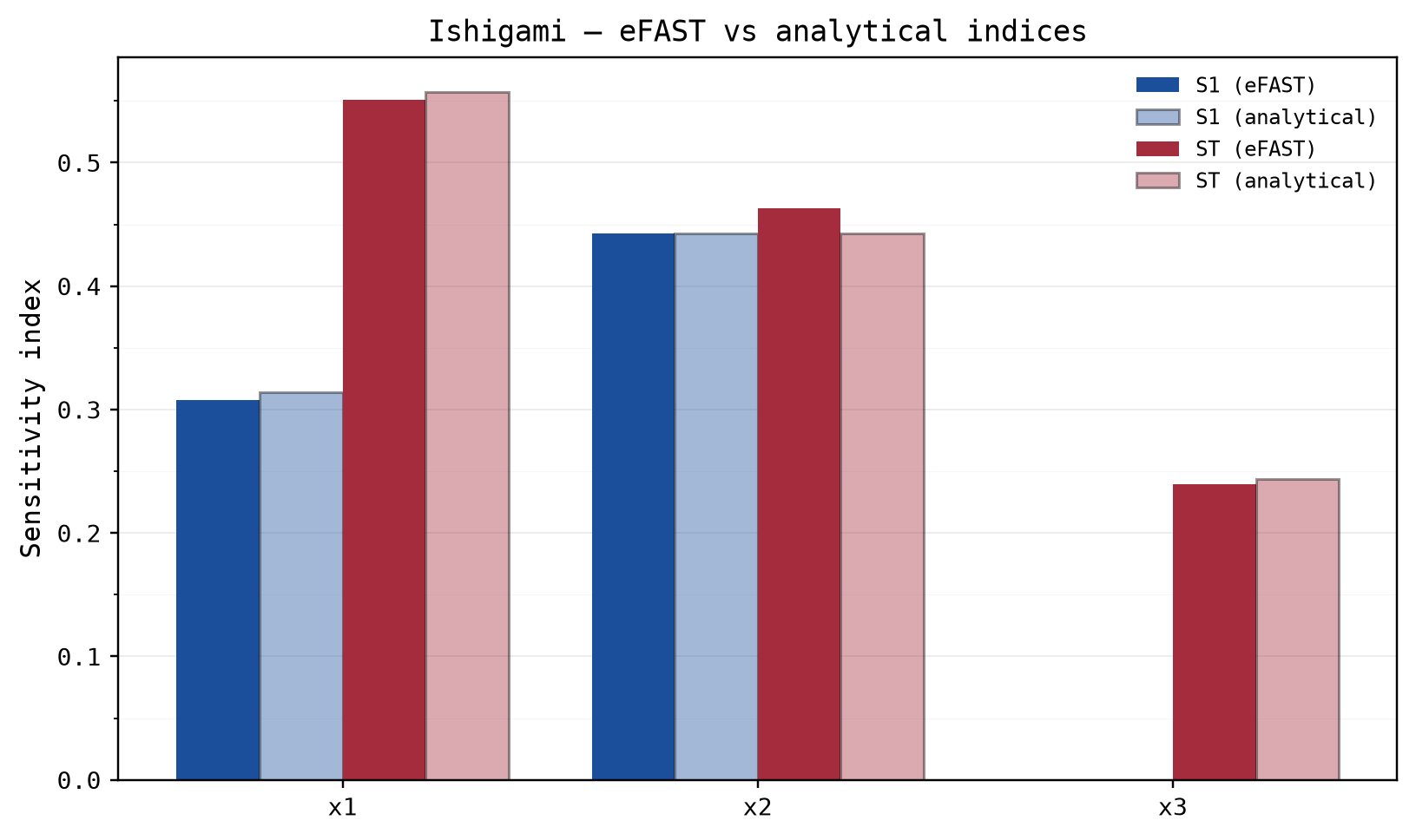
S1: [3.0759001e-01 4.4247049e-01 3.4844247e-10]
ST: [0.550743   0.46297276 0.23925918]
exact S1: [0.31390519 0.44241114 0.        ]
exact ST: [0.55758886 0.44241114 0.24368366]

Ishigami has closed-form indices, so you can read the error directly. S1 is right to about 0.006 and ST to about 0.02. x3 gets S1 = 3e-10, which is zero to float precision, and ST = 0.239 against an exact 0.244. That gap between S1 and ST for x3 is the entire signal for that input: x3 does nothing by itself and a quarter of the variance by interacting with x1.

Compare S1 and ST entry by entry. Equal means the input acts alone. ST much larger means interaction, unattributed. The design cost was 12288 runs: 4096 per curve, three curves.

omega_0 and M come back on the result so a saved analysis records how it was made.

Choosing n_per_curve

The whole budget is n_per_curve * D, so this is the only cost decision. Sweep it once on a cheap model and look for the point where the indices stop moving.

import numpy as np

for n in (129, 257, 513, 1025, 4096):
    s = efast.sample(PROBLEM, n_per_curve=n, seed=42, verbose=False)
    r = efast.analyze(s, evaluate(jnp.asarray(s.samples)), verbose=False)
    print(f"n_per_curve={n:5d} runs={s.n_runs:6d} omega_0={r.omega_0:4d} "
          f"ST={np.round(np.asarray(r.ST), 4)}")
print("exact ST                                    ", np.round(ANALYTICAL_ST, 4))

n_per_curve=  129 runs=   387 omega_0=  16 ST=[0.5135 0.3872 0.2352]
n_per_curve=  257 runs=   771 omega_0=  32 ST=[0.5388 0.4864 0.2356]
n_per_curve=  513 runs=  1539 omega_0=  64 ST=[0.539  0.4863 0.2358]
n_per_curve= 1025 runs=  3075 omega_0= 128 ST=[0.5389 0.4862 0.2357]
n_per_curve= 4096 runs= 12288 omega_0= 511 ST=[0.5507 0.463  0.2393]

This is the trap, and it is worth staring at. From 257 to 1025 the indices are stable to four decimals. They look converged. They are not: ST for x2 sits at 0.486 against an exact 0.442, and only the 4096 run pulls it back towards the truth. A power-of-two-plus-one curve length locks the frequency plan into the same integer relationships across all three of those runs, so they repeat each other's bias instead of averaging it away.

So a stable answer across nearby n_per_curve values is not evidence of accuracy. Change n_per_curve by a large factor rather than a small one, and change it to a length that is not an integer multiple of the previous one. ST summing to well over 1 across inputs is the other cheap check. Here 0.539 + 0.486 + 0.236 = 1.26 at the plateau against 1.25 at 4096 and 1.24 exact, so that check does not catch it either. The honest advice is to spend the runs.

Below the minimum the sampler refuses rather than reusing a frequency:

ValueError: n_per_curve must be >= 4*M^2*(D-1) + 1 = 129 for D = 3 parameters at M = 4, got 128. Below that the D-1 complementary frequencies cannot all be distinct, so non-focal parameters would share a frequency and become indistinguishable along the curve. Raise n_per_curve to at least 129 (costing 387 model runs) or lower M.

Two inputs on the same frequency also share the curve's phase, so their columns are literally identical and no analysis could separate them. That is a silent bias, not a degraded estimate, so it raises.

Choosing M

M defaults to 4 and rarely needs changing, but you cannot judge that without knowing what it does. Here is the frequency plan for D = 3 and n_per_curve = 4097 at four values of M:

M	omega_0	carriers for the other 2 inputs	analysis band
1	2048	1, 1024	1 to 1024
2	1024	1, 256	1 to 512
4	512	1, 64	1 to 256
8	256	1, 16	1 to 128

Look at the top carrier in each row. At M = 1 it is 1024, whose second harmonic is 2048, exactly omega_0. At M = 2 the carrier is 256 and its fourth harmonic is 1024, again exactly omega_0. That is not a coincidence: by construction the top carrier sits at omega_0 / (2 * M), so its 2M-th harmonic always lands on the focal frequency. What M buys you is that the colliding harmonic is a higher one, and higher harmonics carry less power. That is why it is called the interference factor.

for M in (1, 2, 4, 8):
    s = efast.sample(PROBLEM, n_per_curve=4097, M=M, seed=42, verbose=False)
    r = efast.analyze(s, evaluate(jnp.asarray(s.samples)), verbose=False)
    print(f"M={M}  omega_0={r.omega_0:4d}  "
          f"S1={np.round(np.asarray(r.S1), 4)}  ST={np.round(np.asarray(r.ST), 4)}")
print("exact       S1=", np.round(ANALYTICAL_S1, 4), "ST=", np.round(ANALYTICAL_ST, 4))

M=1  omega_0=2048  S1=[0.3175 0.0854 0.    ]  ST=[0.3758 0.1849 0.    ]
M=2  omega_0=1024  S1=[0.2592 0.0034 0.5562]  ST=[0.4489 0.3828 0.6541]
M=4  omega_0= 512  S1=[0.3122 0.4408 0.0289]  ST=[0.5389 0.4862 0.2357]
M=8  omega_0= 256  S1=[0.3134 0.4424 0.0025]  ST=[0.5561 0.4483 0.2444]
exact       S1= [0.3139 0.4424 0.    ] ST= [0.5576 0.4424 0.2437]

M = 2 reports S1 = 0.556 for x3, whose true first-order index is exactly zero. Every number in that row is inside [0, 1], no warning fires, and the ranking is wrong. This is what a silent aliasing failure looks like.

M = 1 fails for a second, separate reason. It credits the focal input only with the power at omega_0 itself. Ishigami's x2 term is 7 * sin(x2)^2, which is 3.5 * (1 - cos(2*x2)), so all of its power sits at twice the fundamental. At M = 1 that harmonic is never counted, and S1 for x2 comes out 0.085 instead of 0.442. Any input whose response is not close to a pure sine spreads power across several harmonics, and M has to be large enough to collect them.

Leave M = 4. Raise it to 8 if you can afford the longer curve it demands and the response is sharply nonlinear. Never lower it.

Higher dimensions: the Sobol G-function

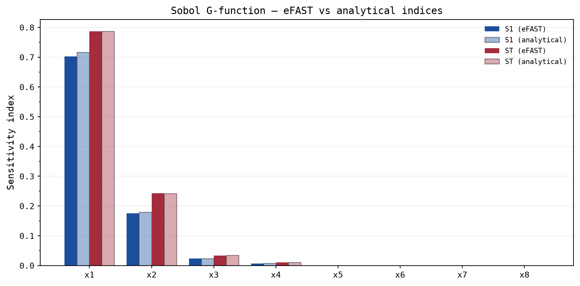
The Sobol G-function is the standard high-dimensional benchmark: g(x) = prod_j (|4*x_j - 2| + a_j) / (1 + a_j), a product of independent factors on [0, 1]^D. The importance vector a sets each input's influence directly: a_j = 0 is maximally influential, a_j = 99 nearly inert. The benchmark's default coefficients are (0, 1, 4.5, 9, 99, 99, 99, 99), so the last four inputs should come out with bars sitting near zero.

import jax.numpy as jnp
from jaxgsa import efast
from jaxgsa.benchmarks.sobol_g import PROBLEM, evaluate

samples = efast.sample(PROBLEM, n_per_curve=4096, M=4, seed=123)
Y = evaluate(jnp.asarray(samples.samples))
result = efast.analyze(samples, Y)
print(result)

jaxgsa.efast.sample: D=8, n_curves=8, n_per_curve=4096, n_runs=32768, M=4, omega_0=511
jaxgsa.efast.analyze
  problem: D=8 (x1, x2, x3, x4, x5, x6, x7, x8)
    marginals: uniform=8
    correlation: independent
    output: N=32768 runs, T=1 x K=1 output slice
    invalid: none found in 8 search curves (policy 'raise')
  timing:
    estimator (includes compile on the first call): 0.533 s
    slice_chunk_size: auto (resolved from the memory budget)
    omega_0: 511, M: 4
  results: top 5 of 8 parameters by ST
    1. x1  ST=0.7874
    2. x2  ST=0.2424
    3. x3  ST=0.03381
    4. x4  ST=0.01047
    5. x7  ST=0.0001825
EFASTResult(S1=(8,), ST=(8,), omega_0=511, M=4)

Eight curves, so the bill is 8 * 4096 = 32768 runs, and the reading follows the coefficients: x1 dominates at ST = 0.787, x2 is moderate, x3 and x4 are weak, and the a = 99 tier comes in at ST = 0.0002 or below (the summary shows x7 at 0.00018). eFAST found the "safe to fix" tier without being told which inputs those were.

There is no confidence interval, and there is no n_bootstrap

efast.analyze takes no n_bootstrap keyword. This is a property of the design.

A bootstrap resamples the unit of observation with replacement. For eFAST that unit is the search curve, and the design has exactly one per input, so there is nothing to resample. Dropping points from within a curve does not help either: the estimator is a discrete Fourier transform of an evenly spaced sweep, so removing a point does not shrink the sample, it changes which frequencies the transform can even see. The number you would get back would be an index of a different design.

What you can do is draw several designs with different random phase shifts and compare.

STs = []
for seed in range(8):
    s = efast.sample(PROBLEM, n_per_curve=1025, seed=seed, verbose=False)
    STs.append(np.asarray(efast.analyze(s, evaluate(jnp.asarray(s.samples)), verbose=False).ST))
STs = np.stack(STs)
print("mean:", np.round(STs.mean(0), 4))
print("min: ", np.round(STs.min(0), 4))
print("max: ", np.round(STs.max(0), 4))

mean: [0.5353 0.488  0.2398]
min:  [0.5228 0.4861 0.2349]
max:  [0.539  0.4894 0.2445]

Be careful with what that buys you. The spread on x2 is 0.4861 to 0.4894, a width of 0.003, while the exact answer is 0.4424 and sits nowhere near the range. A phase ensemble measures sensitivity to the phase and nothing else. The error that dominates at this curve length is the frequency-plan bias from the previous section, and every member of the ensemble shares it. Treat the spread as a lower bound on the error, never as an interval around the truth. If you want a real interval on a variance-based index, use the Sobol workflow, which bootstraps over independent Saltelli groups.

Multi-output example

Y of shape (n_runs, K) gives indices of shape (K, D). Extra outputs cost no extra model runs, so return everything you might want to analyze.

import jaxgsa

problem = jaxgsa.Problem.from_dict(
    {"amplitude": (0.5, 2.0), "frequency": (1.0, 5.0), "damping": (0.01, 0.5)},
    output_names=("displacement", "velocity"),
)


def multi_output_model(X):
    amp, freq, damping = X[:, 0], X[:, 1], X[:, 2]
    return jnp.stack(
        [
            amp * jnp.sin(freq) * jnp.exp(-damping),
            amp * jnp.cos(freq) * jnp.exp(-damping),
        ],
        axis=-1,
    )


samples = efast.sample(problem, n_per_curve=1025, seed=42)
Y = multi_output_model(jnp.asarray(samples.samples))
result = efast.analyze(samples, Y)
print("S1:\n", result.S1)
print("ST:\n", result.ST)

jaxgsa.efast.sample: D=3, n_curves=3, n_per_curve=1025, n_runs=3075, M=4, omega_0=128
jaxgsa.efast.analyze
  problem: D=3 (amplitude, frequency, damping)
    marginals: uniform=3
    correlation: independent
    output: N=3075 runs, T=1 x K=2 output slices
    invalid: none found in 3 search curves (policy 'raise')
  timing:
    estimator (includes compile on the first call): 0.1729 s
    slice_chunk_size: auto (resolved from the memory budget)
    omega_0: 128, M: 4
  results: top 3 of 3 parameters by ST, mean over 2 output slices
    1. frequency  ST=0.9399
    2. amplitude  ST=0.1488
    3. damping    ST=0.03014
S1:
 [[9.0630504e-04 8.7189776e-01 1.2745459e-04]
 [9.2660636e-02 7.7746618e-01 1.5859913e-02]]
ST:
 [[0.10700202 0.9990047  0.01994336]
 [0.19054425 0.8807914  0.04033279]]

Row 0 is displacement and row 1 is velocity, in output_names order. Read amplitude on the first output: S1 = 0.0009 and ST = 0.107. Amplitude multiplies the whole expression, so on its own it explains nothing about the variance of sin(frequency), and all of its effect is interaction. The top-k table averages over output slices, which is fine for a glance and wrong to quote.

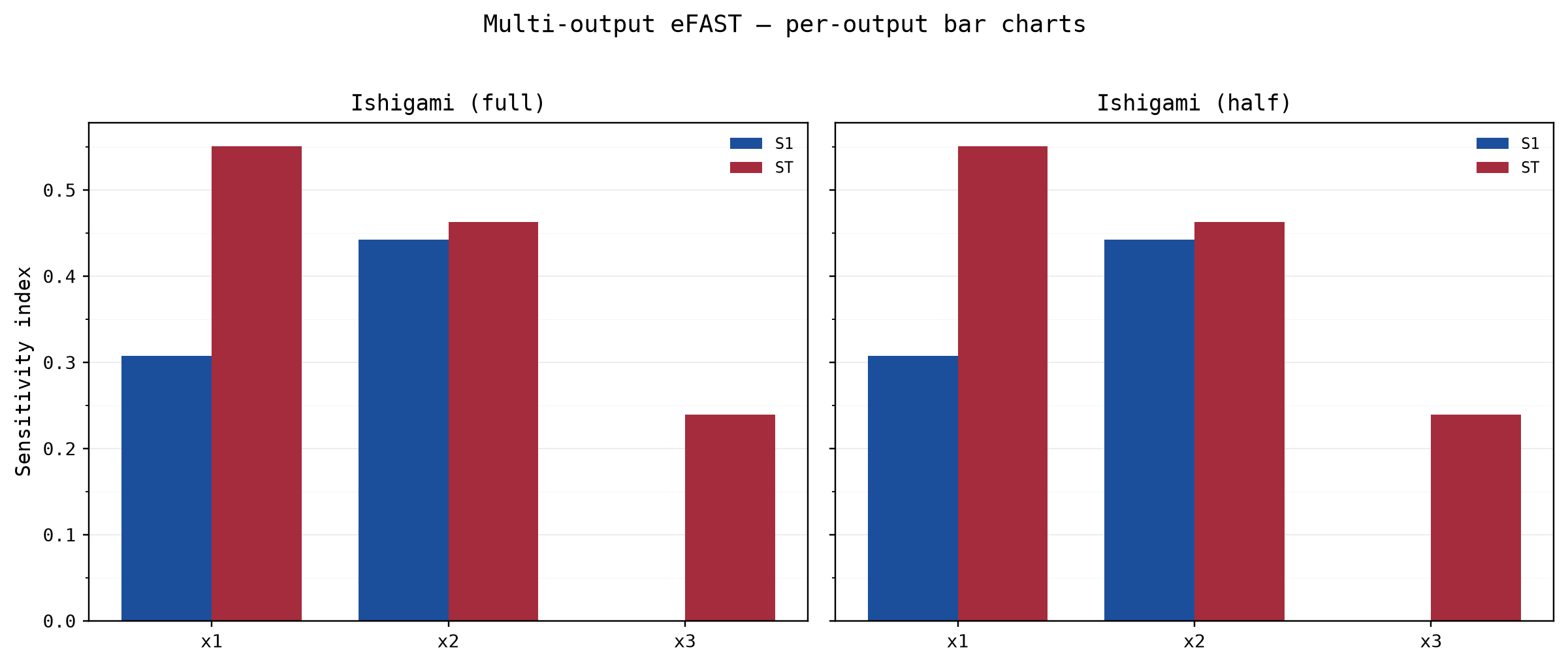
A cheaper way to build a second output is to scale the first one. The script's multi-output demo stacks the full Ishigami output with its half-amplitude copy:

import jax.numpy as jnp
from jaxgsa import efast
from jaxgsa.benchmarks import ishigami

samples = efast.sample(ishigami.PROBLEM, n_per_curve=4096, M=4, seed=7)
Y_full = ishigami.evaluate(jnp.asarray(samples.samples))
Y_multi = jnp.stack([Y_full, 0.5 * Y_full], axis=-1)  # (n_runs, 2)

result = efast.analyze(samples, Y_multi)
print(result)

jaxgsa.efast.sample: D=3, n_curves=3, n_per_curve=4096, n_runs=12288, M=4, omega_0=511
jaxgsa.efast.analyze
  problem: D=3 (x1, x2, x3)
    marginals: uniform=3
    correlation: independent
    output: N=12288 runs, T=1 x K=2 output slices
    invalid: none found in 3 search curves (policy 'raise')
  timing:
    estimator (includes compile on the first call): 0.6224 s
    slice_chunk_size: auto (resolved from the memory budget)
    omega_0: 511, M: 4
  results: top 3 of 3 parameters by ST, mean over 2 output slices
    1. x1  ST=0.5507
    2. x2  ST=0.463
    3. x3  ST=0.2393
EFASTResult(S1=(2, 3), ST=(2, 3), omega_0=511, M=4)

A constant scale cancels in every variance ratio, so both slices return the same indices — the top-k summary is unchanged from the scalar case. That makes the scaled copy a way to check the multi-output path, not a way to learn something new about the model.

Time-series example

Y of shape (n_runs, T, K) gives indices of shape (T, K, D). Same design, same cost.

import numpy as np

time_values = np.linspace(0.25, 5.0, 20)


def time_series_model(X):
    amp, freq, damping = X[:, 0, None], X[:, 1, None], X[:, 2, None]
    tt = jnp.asarray(time_values)[None, :]
    env = amp * jnp.exp(-damping * tt)
    return jnp.stack(
        [env * jnp.sin(2 * jnp.pi * freq * tt), env * jnp.cos(2 * jnp.pi * freq * tt)],
        axis=-1,
    )


samples = efast.sample(problem, n_per_curve=1025, seed=42)
Y = time_series_model(jnp.asarray(samples.samples))
result = efast.analyze(samples, Y)

print("S1 shape:", result.S1.shape, "ST shape:", result.ST.shape)
print("damping ST, displacement, t = 0.25 / 2.5 / 5.0:",
      np.round(np.asarray(result.ST[[0, 9, 19], 0, 2]), 4))
print("amplitude ST, same times:  ",
      np.round(np.asarray(result.ST[[0, 9, 19], 0, 0]), 4))

jaxgsa.efast.sample: D=3, n_curves=3, n_per_curve=1025, n_runs=3075, M=4, omega_0=128
jaxgsa.efast.analyze
  problem: D=3 (amplitude, frequency, damping)
    marginals: uniform=3
    correlation: independent
    output: N=3075 runs, T=20 x K=2 output slices
    invalid: none found in 3 search curves (policy 'raise')
  timing:
    estimator (includes compile on the first call): 0.201 s
    slice_chunk_size: auto (resolved from the memory budget)
    omega_0: 128, M: 4
  results: top 3 of 3 parameters by ST, mean over 40 output slices
    1. damping    ST=0.8998
    2. frequency  ST=0.875
    3. amplitude  ST=0.108
S1 shape: (20, 2, 3) ST shape: (20, 2, 3)
damping ST, displacement, t = 0.25 / 2.5 / 5.0: [0.0012 0.9944 0.9945]
amplitude ST, same times:   [0.1073 0.1066 0.1473]

Damping goes from 0.0012 to 0.994. At t = 0.25 the exponential has barely started and damping is irrelevant; by t = 2.5 it controls essentially everything. Any single-time ranking of this model is a statement about that time and no other. Plot the index curves before you rank.

The failure mode here is a time step where the output has no variance at all. If the grid had started at t = 0, every sample would give displacement = 0 exactly, there would be no variance to divide up, and the indices for that slice would be NaN. eFAST says so twice, once per slice and once per curve:

JaxgsaWarning: jaxgsa.efast.analyze: 1/40 output slice(s) have zero variance [(t=0, k=0 ('displacement'))] — corresponding indices will be NaN
JaxgsaWarning: jaxgsa.efast: 3 search-curve/output slice(s) have zero variance — corresponding indices will be NaN

A NaN slice also poisons the mean in the verbose top-k table, so the summary will report ST=nan for every input. Drop the degenerate time steps before you analyze, or start the grid past them.

Time series on a damped oscillator

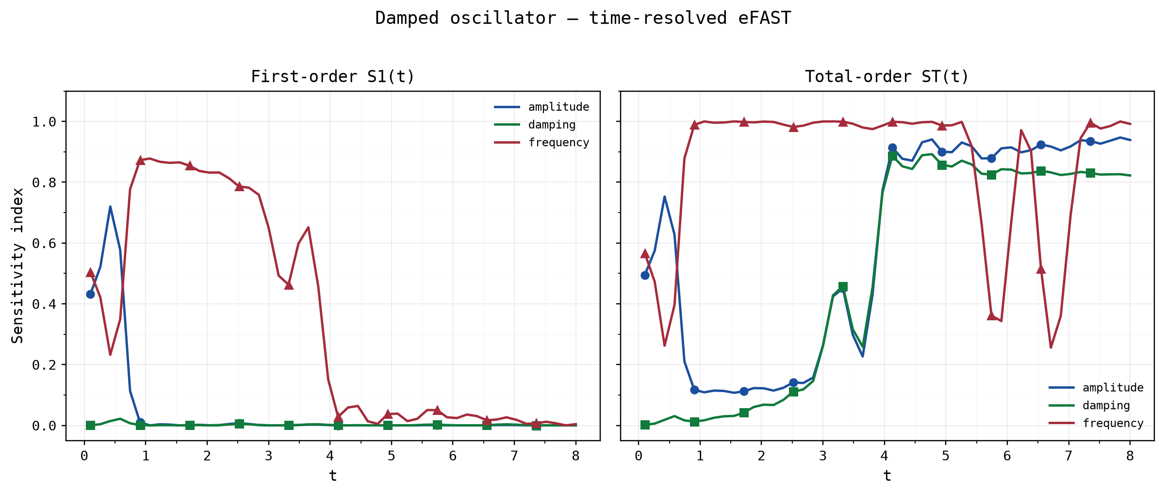
The script's time-series demo is a single-output damped oscillator, y(t) = A * exp(-gamma * t) * sin(omega * t), with amplitude on (0.5, 2.0), damping on (0.1, 0.5) and frequency on (1.0, 5.0), sampled at 50 steps of t from 0.1 to 8.0.

import jax.numpy as jnp
from jaxgsa import Problem, efast

problem = Problem.from_dict(
    {"amplitude": (0.5, 2.0), "damping": (0.1, 0.5), "frequency": (1.0, 5.0)}
)

times = jnp.linspace(0.1, 8.0, 50)


def damped_oscillator(X, ts):
    amplitude = X[:, 0:1]
    gamma = X[:, 1:2]
    omega = X[:, 2:3]
    return amplitude * jnp.exp(-gamma * ts[None, :]) * jnp.sin(omega * ts[None, :])


samples = efast.sample(problem, n_per_curve=4096, M=4, seed=99)
Y = damped_oscillator(jnp.asarray(samples.samples), times)
Y = Y[..., None]  # (n_runs, T, 1)
result = efast.analyze(samples, Y)
print(result)

jaxgsa.efast.sample: D=3, n_curves=3, n_per_curve=4096, n_runs=12288, M=4, omega_0=511
jaxgsa.efast.analyze
  problem: D=3 (amplitude, damping, frequency)
    marginals: uniform=3
    correlation: independent
    output: N=12288 runs, T=50 x K=1 output slices
    invalid: none found in 3 search curves (policy 'raise')
  timing:
    estimator (includes compile on the first call): 0.2865 s
    slice_chunk_size: auto (resolved from the memory budget)
    omega_0: 511, M: 4
  results: top 3 of 3 parameters by ST, mean over 50 output slices
    1. frequency  ST=0.8588
    2. amplitude  ST=0.5996
    3. damping    ST=0.4983
EFASTResult(S1=(50, 1, 3), ST=(50, 1, 3), omega_0=511, M=4)

The Y[..., None] reshape adds the trailing K = 1 axis, so the analyzer sees (n_runs, T, 1) and returns indices of shape (T, K, D) = (50, 1, 3) — the same convention the shape rules describe for a single named output. The physics shows up in the time course: amplitude controls the early envelope. At t = 0.1 the exponential has barely moved, and the dataset print shows amplitude's S1 opening at 0.432 while damping's opens at 0.0005. Damping decides the decay later, as exp(-gamma * t) collapses; frequency carries the oscillation itself, which is why it holds the largest mean ST over the whole window (0.859).

Saving a design

EFASTSamples.save() and .load() round-trip the design through an NPZ file, including n_per_curve and M. Use it when the model runs somewhere the analysis does not.

samples.save("efast_design.npz")
reloaded = efast.EFASTSamples.load("efast_design.npz")
print(reloaded.n_per_curve, reloaded.M, reloaded.samples.shape)

1025 4 (3075, 3)

The row order is the contract. Curve i is rows i*n_per_curve : (i+1)*n_per_curve, and the analysis will silently attribute power to the wrong input if a downstream job reorders or shuffles them.

Categorical inputs are refused

ValueError: jaxgsa.efast.sample requires continuous (orderable) inputs, but parameters ['material'] are categorical. Use jaxgsa.sobol.sample (the Saltelli column-swap scheme is distribution-agnostic; it requires a problem with no declared correlation), or analyze given data with jaxgsa.optimal_transport, jaxgsa.borgonovo or jaxgsa.pawn.

The search curve is a continuous sweep: an input slides smoothly through its range at a fixed frequency, and the Fourier transform reads the smoothness. A categorical input has level codes with no order, so "sweep it sinusoidally" has no meaning, and any answer would be an artefact of how the levels happened to be numbered. Sobol works instead, because its column-swap scheme only ever substitutes whole values and never interpolates between them. eFAST also refuses a problem with a declared correlation, for the same reason: the curve moves the inputs independently by construction.

Shape rules

n_runs = n_per_curve * D is the design's total row count (samples.n_runs). analyze rejects any Y with a different leading dimension.

• (n_runs,) is scalar output.
• (n_runs, K) is K output variables with no time dimension.
• (n_runs, T, K) is T time steps and K outputs.
• Without problem.output_names, a 2D array is always read as (n_runs, K).
• With exactly one name in problem.output_names, a 2D array is read as (n_runs, T), the timepoints of that single output, and flows through as (n_runs, T, 1). A pre-reshaped (n_runs, T, 1) array works too.

Y shape	S1 / ST shape
(n_runs,)	(D,)
(n_runs, K)	(K, D)
(n_runs, T, K)	(T, K, D)

D is always the last axis.

Practical caveats

• No S2. Use the Sobol workflow for pairwise interaction estimates.
• No n_bootstrap, for the reason given above.
• M is fixed at sample() time and travels inside EFASTSamples, so it can never be mismatched at analyze() time.
• n_per_curve >= 4*M^2*(D-1) + 1. At the default M = 4 that is 129 for D = 3 and 577 for D = 10, and the total run count is D times that.
• Indices outside [0, 1] mean too few samples or near-zero output variance. Indices inside [0, 1] mean nothing on their own, as the M = 2 row above shows.
• on_invalid="drop" is not available. Only "raise" (the default) and "propagate". Dropping a point from a Fourier sweep changes the estimator.
• to_dataset(time_coords=...) gives a labeled xarray.Dataset with omega_0 and M in its attributes.

See also

• Basic example for the Sobol workflow, with S2 and real confidence intervals.
• Morris for a much cheaper screen when a ranking is all you need.
• Multi-output and time series for the same shape conventions on Sobol and HDMR.
• xarray labeled output for named access by parameter, output and time.
• Methods for the theory and the method comparison.