Multi-Output & Time-Series

jaxgsa reads the meaning of your output array from its rank alone. It does not guess, and it does not transpose. (N,) is a scalar output, (N, K) is K outputs at one instant, and (N, T, K) is K outputs over T timepoints. N is the number of model runs and D is the number of input parameters.

Two axes of the same length are where this bites, and a time axis and an output axis are both just integers. The last two sections give the full table of what is accepted, what raises, and the one case that is accepted and means something other than you intended.

The full script is examples/dynamic_gsa.py, run with uv run python examples/dynamic_gsa.py.

One model, two layouts

A damped oscillator with four inputs, returning displacement and velocity at 40 timepoints. Displacement carries an additive offset term; velocity does not. That asymmetry is the check later on.

python

import jax.numpy as jnp
import numpy as np
import jaxgsa

problem = jaxgsa.Problem.from_dict(
    {
        "amplitude": (0.5, 2.0),
        "frequency": (1.0, 5.0),
        "damping": (0.01, 0.5),
        "offset": (-1.0, 1.0),
    },
    output_names=("displacement", "velocity"),
)

time_values = np.linspace(0.0, 5.0, 40)


def oscillator(X):
    amp = X[:, 0, None]
    freq = X[:, 1, None]
    damping = X[:, 2, None]
    offset = X[:, 3, None]
    tt = jnp.asarray(time_values)[None, :]

    displacement = amp * jnp.sin(2 * jnp.pi * freq * tt) * jnp.exp(-damping * tt) + offset
    velocity = amp * jnp.cos(2 * jnp.pi * freq * tt) * jnp.exp(-damping * tt)

    return jnp.stack([displacement, velocity], axis=-1)  # (N, T, K)


design = jaxgsa.sobol.sample(problem, n_samples=2048, seed=42)
X = jnp.asarray(design.samples)

Y_time = oscillator(X)         # (N, T, K) = (2560, 40, 2)
Y_snapshot = Y_time[:, -1, :]  # (N, K)    = (2560, 2)

time_result = jaxgsa.sobol.analyze(design, Y_time)
snapshot_result = jaxgsa.sobol.analyze(design, Y_snapshot)

jnp.stack(..., axis=-1) is the line that makes the layout work. Stack outputs on the last axis and you get (N, T, K) for free. Stack them anywhere else and you will spend the rest of this page fighting the shape rules.

text

jaxgsa.sobol.sample: D=4, mode=second-order, base_n=256, requested_runs>=2048, n_runs=2560, n_expanded=2560, duplicates_removed=0 (0.0%), scramble=True
jaxgsa.sobol.analyze
  problem: D=4 (amplitude, frequency, damping, offset)
    marginals: uniform=4
    correlation: independent
    output: N=2560 runs, T=40 x K=2 output slices
    invalid: none found in 256 Saltelli groups (policy 'raise')
  timing:
    estimators (includes compile on the first call): 0.4486 s
    slice_chunk_size: 80 (resolved from the memory budget)
    estimator: saltelli-jansen
  results: top 4 of 4 parameters by ST, mean over 80 output slices
    1. frequency  ST=0.7365
    2. offset     ST=0.2497
    3. amplitude  ST=0.09106
    4. damping    ST=0.08931

T=40 x K=2 output slices is the line that confirms jaxgsa read your array the way you meant it. Check it before you read any index. The ranking underneath is a mean over all 80 slices, which is a summary and nothing more. A parameter that dominates for the first ten timepoints and vanishes afterwards averages down to nothing here.

The second call prints T=1 x K=2 output slices for the same reason, and it resolves slice_chunk_size to 2 instead of 80, because there are only 2 slices left to work on.

What comes back

python

np.set_printoptions(precision=3, suppress=True)

print("time S1    ", time_result.S1.shape)
print("snapshot S1", snapshot_result.S1.shape)
print("displacement @ last t:", np.asarray(time_result.S1[-1, 0, :]))
print("velocity     @ last t:", np.asarray(time_result.S1[-1, 1, :]))
print("snapshot displacement:", np.asarray(snapshot_result.S1[0, :]))
print("snapshot velocity    :", np.asarray(snapshot_result.S1[1, :]))

text

time S1     (40, 2, 4)
snapshot S1 (2, 4)
displacement @ last t: [-0.003  0.161 -0.018  0.663]
velocity     @ last t: [ 0.021  0.689 -0.07   0.   ]
snapshot displacement: [-0.003  0.161 -0.018  0.663]
snapshot velocity    : [ 0.021  0.689 -0.07   0.   ]

The index array mirrors the output array with N replaced by D and moved to the end. (N, T, K) in gives (T, K, D) out, 320 numbers. (N, K) in gives (K, D) out. The parameter order inside the last axis is the declaration order from from_dict(), so amplitude, frequency, damping, offset.

The snapshot rows are identical to the last-timepoint rows, to every digit printed. They are the same data reaching the same estimator by two routes. If you ever slice a time result and get something different from analysing the slice directly, the layout was misread somewhere.

Now read the numbers. For velocity, offset scores exactly 0.000. That is structural rather than a small estimate. Velocity has no offset term, so the estimator recovers a hard zero. Use a known-absent input this way whenever you can. It is the cheapest possible check that your outputs are lined up with your design.

For displacement, offset is the largest contributor at 0.663 and frequency is second at 0.161. At t = 0 the split is very different:

python

print("displacement S1 for offset,    t = 0 / 2.56 / 5:", np.asarray(time_result.S1[[0, 20, 39], 0, 3]))
print("displacement S1 for amplitude, t = 0 / 2.56 / 5:", np.asarray(time_result.S1[[0, 20, 39], 0, 0]))

text

displacement S1 for offset,    t = 0 / 2.56 / 5: [0.953 0.499 0.663]
displacement S1 for amplitude, t = 0 / 2.56 / 5: [0.   0.008 -0.003]

At t = 0 the sine is zero, so displacement is the offset and nothing else, and S1 says 0.953. By the middle of the window the oscillation has taken half the variance. This is the reason to keep the time axis rather than analyse a summary statistic. A single number for the whole trajectory would have reported one blend of these and hidden the fact that the driver changes.

amplitude scores near zero throughout, and at the last timepoint it is negative, -0.003. A negative Sobol index is impossible, so that is the noise floor. Amplitude only enters multiplied by a sine whose sign flips fast across the frequency range, so its main effect averages out. Its ST is 0.036, which is small but real.

When 256 base points is not enough

The verbose block reported base_n=256, because a second-order design at D=4 spends 10 rows per base point. Look at what that does to the total-order index:

python

print("ST velocity @ last t:", np.asarray(time_result.ST[-1, 1, :]))

text

ST velocity @ last t: [0.103 1.158 0.349 0.   ]

frequency has ST = 1.158. A total-order index is a variance share and cannot exceed 1. Rerunning at n_samples=65536, so base_n=8192, brings it to 0.983. Nothing was fixed. The estimator was simply averaging 256 samples of a quantity that swings hard, because at t = 5 a frequency anywhere in [1, 5] puts the cosine anywhere in [-1, 1].

Two things follow. An index above 1 or below 0 is a sample-size warning, and it is the only free one you get without bootstrapping. And a wildly oscillating output needs far more samples than a smooth one for the same accuracy, so pick n_samples from the roughness of your output, not from D. Confidence intervals from Bootstrap Confidence Intervals give you the same warning for every index rather than only for the ones that overshoot.

Compare three methods across time

This section overlays Sobol, eFAST, and DGSM on one time-resolved model: a coupled damped oscillator

y (t) = A \sin (2 π ω t) e^{- γ t} + κ t e^{- γ t}

with four uniform inputs — amplitude $A \in [0.5, 2.0]$ , frequency $ω \in [1.0, 5.0]$ , damping $γ \in [0.01, 0.5]$ , coupling $κ \in [0.1, 2.0]$ — evaluated at $T = 50$ steps over $t \in [0.1, 10.0]$ . The whole workflow, three estimators on the same model:

python

import jax
import jax.numpy as jnp
import jaxgsa

problem = jaxgsa.Problem.from_dict(
    {
        "amplitude": (0.5, 2.0),
        "frequency": (1.0, 5.0),
        "damping": (0.01, 0.5),
        "coupling": (0.1, 2.0),
    },
)
T = 50
times = jnp.linspace(0.1, 10.0, T)


def oscillator(X):
    """Batched: (N, D) -> (N, T)."""
    amp, freq, damping, coupling = X[:, 0:1], X[:, 1:2], X[:, 2:3], X[:, 3:4]
    t = times[None, :]
    return amp * jnp.sin(2 * jnp.pi * freq * t) * jnp.exp(-damping * t) + coupling * t * jnp.exp(
        -damping * t
    )


# 1. Sobol (Saltelli), first/total-order only
sampling_result = jaxgsa.sobol.sample(problem, n_samples=4096, seed=0, calc_second_order=False)
Y_sobol = oscillator(jnp.asarray(sampling_result.samples))[..., None]  # (N, T) -> (N, T, 1)
sobol_result = jaxgsa.sobol.analyze(
    sampling_result,
    Y_sobol,
    n_bootstrap=200,
    conf_level=0.95,
    ci_method="quantile",
    key=jax.random.key(0),
)

# 2. eFAST on the same model
efast_samples = jaxgsa.efast.sample(problem, n_per_curve=4096, M=4, seed=42)
Y_ef = oscillator(jnp.asarray(efast_samples.samples))[..., None]
efast_result = jaxgsa.efast.analyze(efast_samples, Y_ef)

# 3. DGSM on the unbatched function
def oscillator_unbatched(x):
    """Unbatched: (D,) -> (T,)."""
    amp, freq, damping, coupling = x
    t = times
    return amp * jnp.sin(2 * jnp.pi * freq * t) * jnp.exp(-damping * t) + coupling * t * jnp.exp(
        -damping * t
    )


X_dgsm = jaxgsa.sampling.monte_carlo(problem, n=50_000, seed=7)
dgsm_result = jaxgsa.dgsm.analyze(problem, oscillator_unbatched, jnp.asarray(X_dgsm))

calc_second_order=False keeps the Saltelli design at $(D + 2) \times base_n = 6 \times 1024 = 6144$ runs instead of the 10240 a second-order design would cost, and the trajectory already multiplies the output 50-fold. The [..., None] reshape turns the (N, T) output into (N, T, 1) so the axis is read as time; without it the 50 steps would be read as 50 separate outputs at one instant. The bootstrap adds a 95% quantile interval per index from 200 replicates.

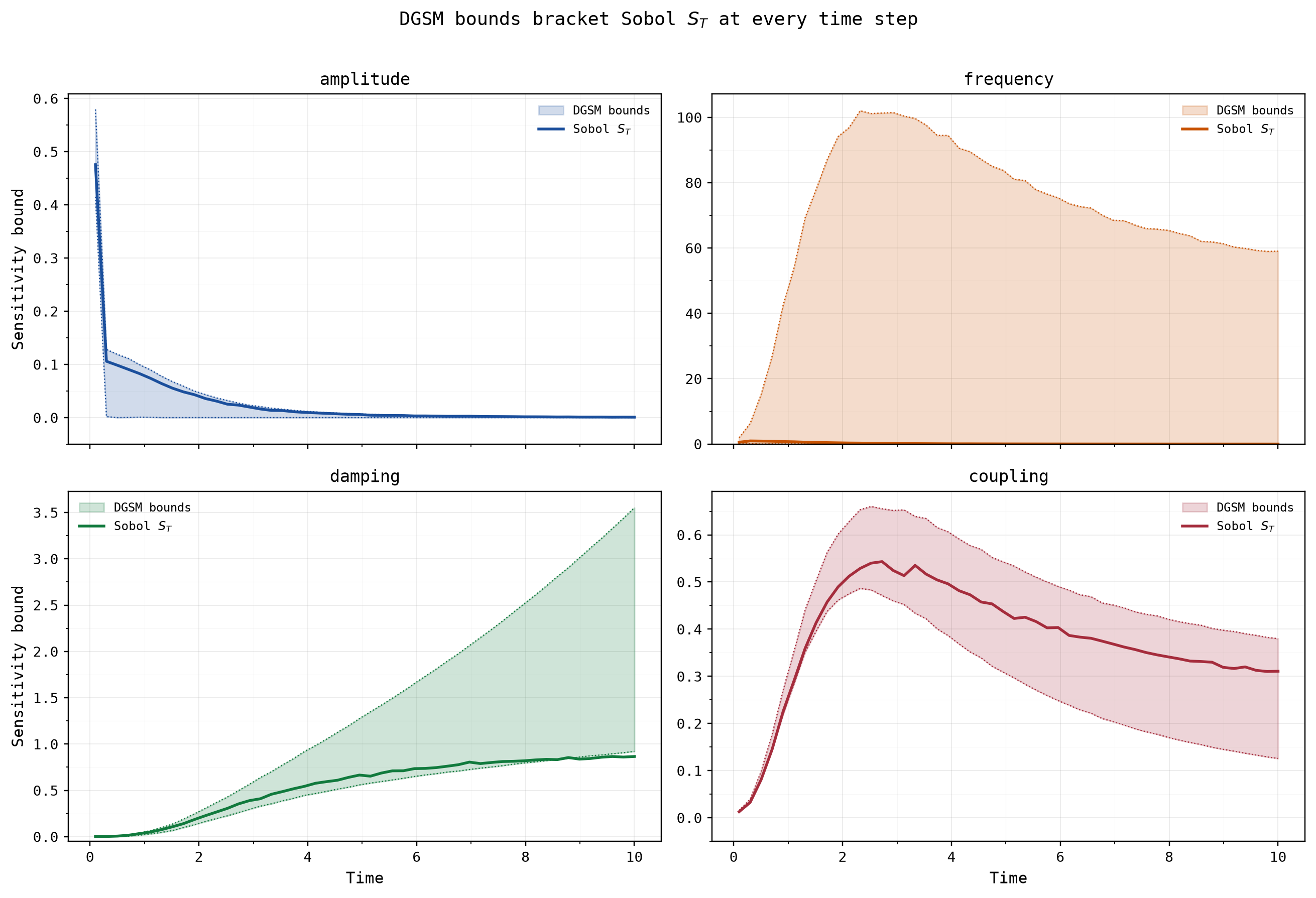
DGSM is the odd one out, and the verbose block says why: with a bare (D,) -> (T,) function, analyze counts every time step as an independent output — the report reads T=1 x K=50 output slices — and returns bounds of shape (50, 4), i.e. (T, D), with gradients: forward-mode autodiff (T*K=50, D=4).

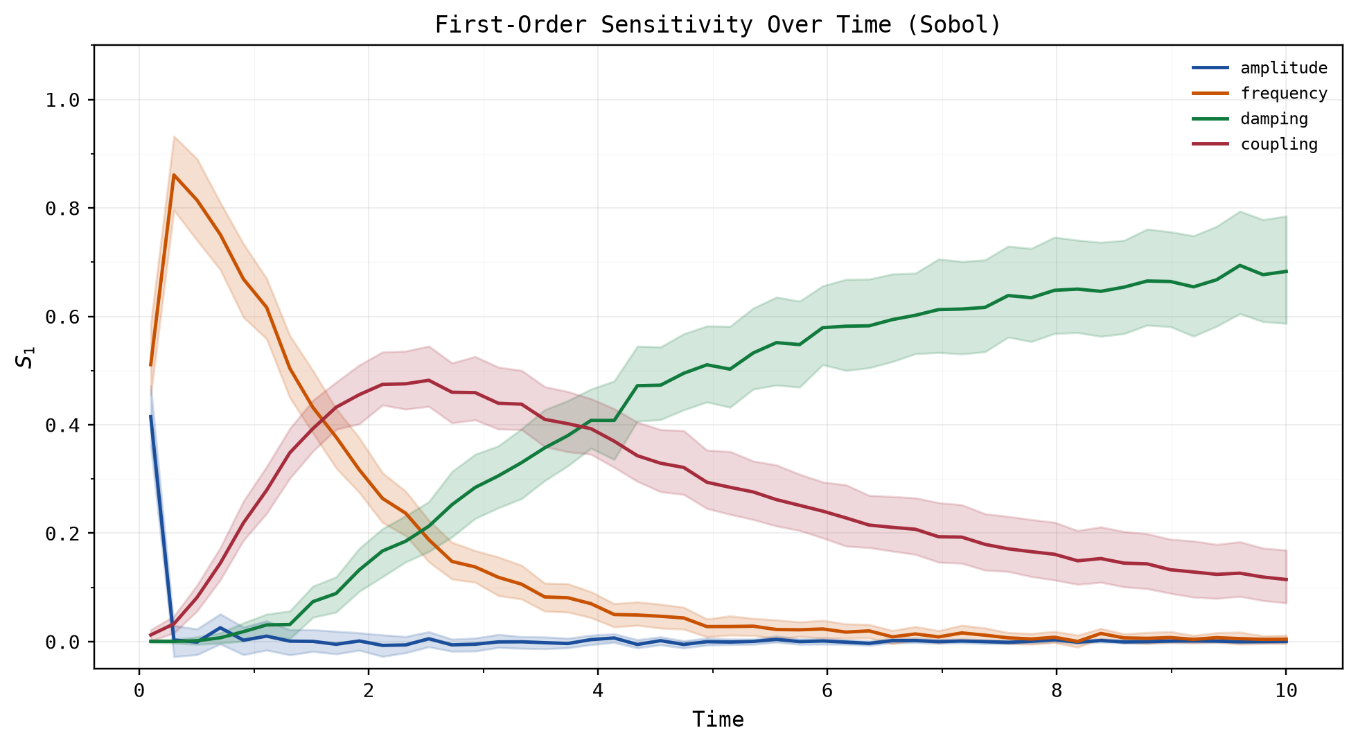
Three phases. The Sobol $S_{T}$ curves split the trajectory into three phases. Numbers are $S_{T}$ in parameter order amplitude, frequency, damping, coupling unless stated.

Early, $t ≲ 2$ : the oscillatory term carries the variance. At $t = 0.1$ , $S_{T} = [0.476, 0.572, 0.001, 0.013]$ : amplitude and frequency share it through $A \sin (2 π ω t)$ , while damping and coupling are negligible because $e^{- γ t} \approx 1$ . Frequency carries the largest mean $S_{1}$ in the window (0.585 over $t < 2$ ; 0.669 at $t = 0.91$ ), coupling's linear $κ t$ term climbs ( $S_{1}$ from 0.012 at $t = 0.1$ to 0.393 at $t = 1.5$ ), and amplitude's main effect washes out once the sine averages over $ω$ ( $S_{1}$ from 0.415 at $t = 0.1$ to 0.003 at $t = 0.91$ ).
Mid, $2 ≲ t ≲ 5$ : coupling and damping overtake frequency. At $t = 3.5$ , $S_{1} = [- 0.002, 0.082, 0.357, 0.410]$ — the envelope decay and the $κ t e^{- γ t}$ term now shape the variance.
Late, $t > 5$ : damping takes over. $S_{1}$ runs 0.62-0.68 and $S_{T}$ 0.79-0.87; at $t = 10.0$ , $S_{T} = [0.001, 0.009, 0.866, 0.311]$ .

A steady-state analysis at a single late time captures only the last phase: at $t = 10.0$ it would report damping 0.866 and coupling 0.311 with frequency and amplitude at the noise floor, and the early story — frequency's lead, coupling's climb — invisible.

First-order Sobol sensitivity S1(t) over time for amplitude, frequency, damping and coupling, with bootstrap 95% confidence bands

Total-order Sobol sensitivity ST(t) over time for the four oscillator inputs, with bootstrap 95% confidence bands

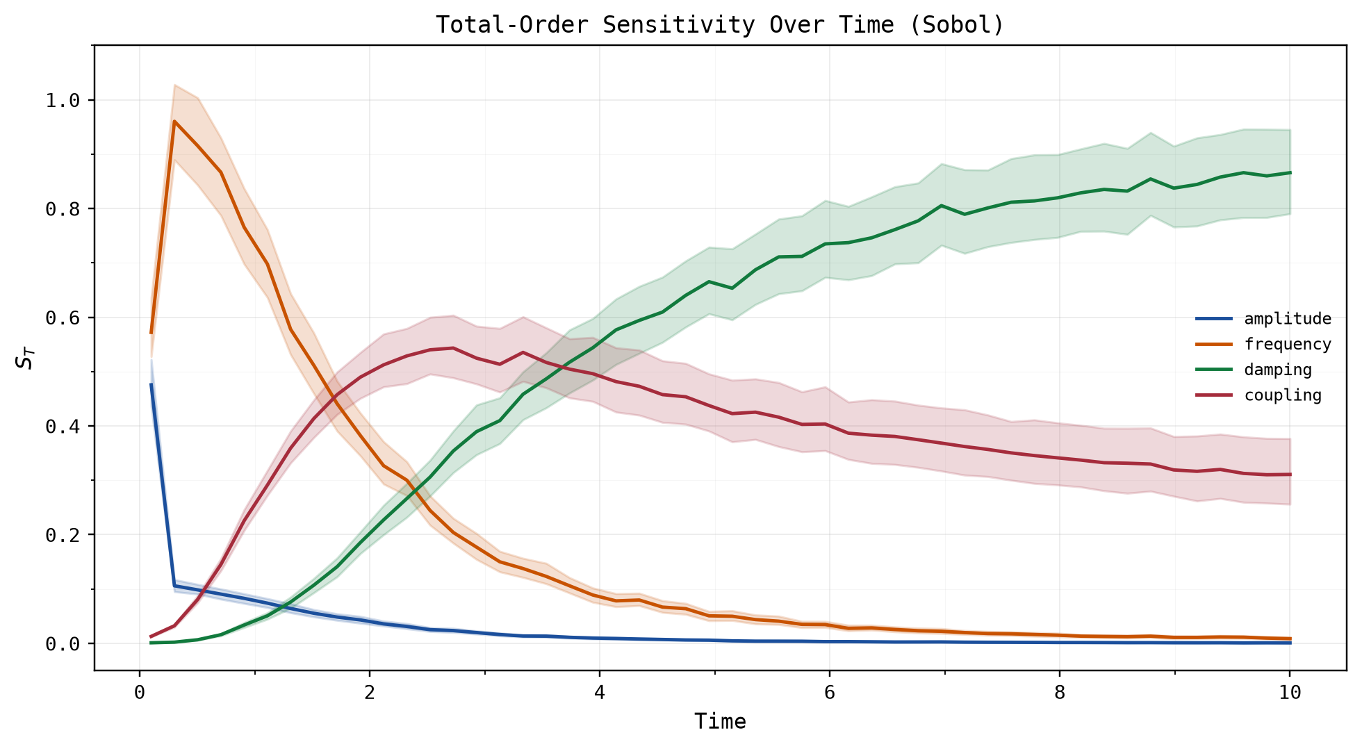
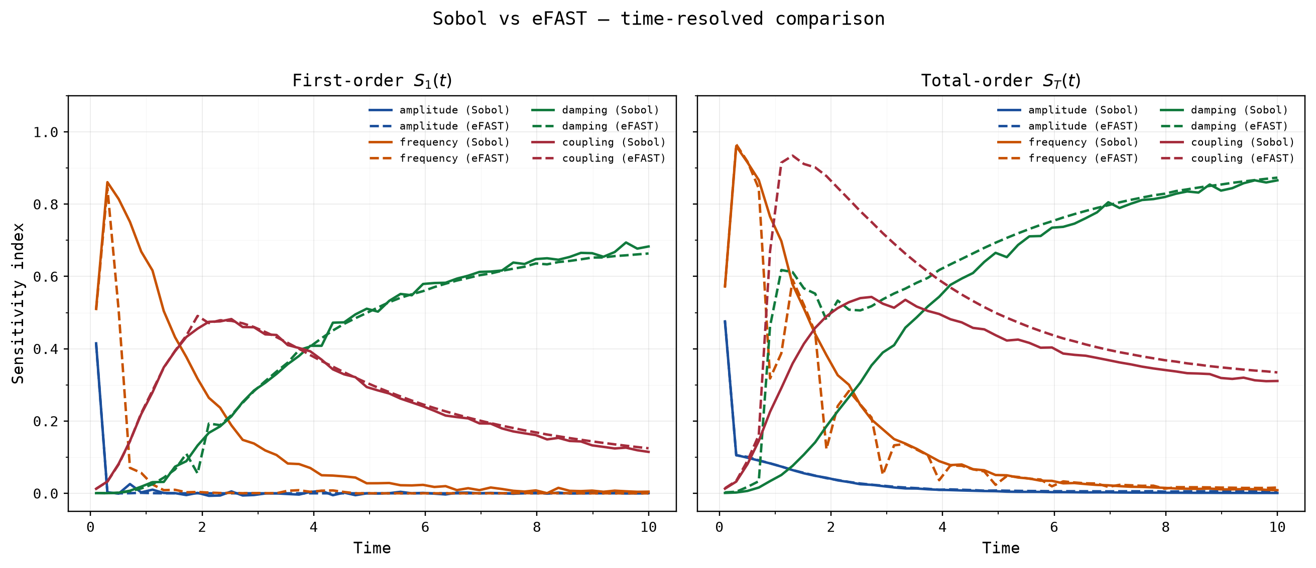
Cross-method agreement. The mean-over-time reports agree on the broad ranking: damping first, amplitude last, with coupling and frequency second and third (Sobol $S_{T}$ 0.5501 / 0.3793 / 0.1884 / 0.0286; eFAST $S_{T}$ 0.6477 / 0.5004 / 0.1627 / 0.0310). DGSM's $ν$ means put frequency second (313.8 / 152.2 / 4.386 / 0.1366): $\partial y / \partial ω$ carries a factor $t$ , so the squared-derivative measure weights the fast term more heavily than its variance share.

Solid Sobol lines and dashed eFAST lines agree where the output is smooth: amplitude everywhere, and the late phase (mean $S_{T}$ over $t > 5$ : damping 0.794 vs 0.808, coupling 0.358 vs 0.390). They diverge in the early transient, where the output oscillates fastest: at $t = 0.91$ Sobol gives frequency $S_{T}$ 0.765 where eFAST gives 0.318, and eFAST's $S_{T}$ for damping and coupling runs far above Sobol's (0.462 vs 0.034, 0.67 vs 0.226). The fast oscillation spreads the frequency input's power across Fourier harmonics, so eFAST's $S_{1}$ for frequency reads 0.057 against Sobol's 0.669 at that step.

Two-panel time series of first-order Sobol indices S1(t) with solid Sobol lines overlaid by dashed eFAST lines

The DGSM bracket tracks the Sobol $S_{T}$ curve through the trajectory and contains all four point estimates at 42 of the 50 steps. The exceptions are the uniform-marginal warning doing its job: the script warns that the Kucherenko-Song lower bound is an estimate, not a strict bound, for uniform marginals, and the misses are lower estimates sitting above the $S_{T}$ point estimate — coupling by $3 \times 10^{- 5}$ at $t = 0.1$ , and damping by 0.3-6% for $t \geq 8.6$ (0.835 vs 0.832 at $t = 8.6$ ; 0.921 vs 0.866 at $t = 10.0$ ). So the bracket is a sanity check, not a proof: it hugs the Sobol curve everywhere and contains it almost everywhere, and the misses are exactly the failure mode the warning names.

2x2 grid of DGSM sensitivity panels, one per oscillator parameter, with the first panel titled amplitude

The full shape table

Every row below was run against a design built from a 4-parameter problem, with N = 2560 and 40 timepoints.

`Y` shape	`problem.output_names`	Result
`(2560,)`	none, or 1 name	`S1` is `(4,)`
`(2560,)`	2 names	`ValueError: output_names length 2 does not match the output axis K=1`
`(2560, 2)`	2 names	`S1` is `(2, 4)`
`(2560, 40, 2)`	2 names	`S1` is `(40, 2, 4)`
`(2560, 40, 1)`	1 name	`S1` is `(40, 1, 4)`
`(2560, 40)`	1 name	`ValueError: output_names length 1 does not match the output axis K=40`
`(2560, 40)`	none	`S1` is `(40, 4)`, and the 40 are read as outputs
`(2, 2560)`	2 names	`ValueError: Y has 2 sample rows but 2560 were expected`
`(2560, 40, 2, 1)`	2 names	`ValueError: Y must be 1-D (N,), 2-D (N, K), or 3-D (N, T, K)`

Four rules cover the table.

The sample axis is always first. A transposed array is caught by the row count, not by an axis-shape heuristic, and there is no warning and no repair. If your model returns (K, N), transpose it yourself.

Rank fixes the meaning. A 2D array is (N, K), always. There is no case in which jaxgsa reads a 2D array as (N, T).

output_names is a hard check, not a label. Its length must equal the size of the last axis, and 1 for a 1D array. Set it and it catches the mistakes in rows 2 and 6 before any compute happens. This is the strongest reason to name your outputs even when you never plan to export a dataset.

Rank above 3 raises immediately.

The one silent case

Row 7 is the one to watch. Pass (N, T) with no output_names and it is accepted as T separate outputs at a single instant.

The index values are unharmed. Sobol treats every slice independently, so analyze(d0, Y_2d).S1 matches analyze(d1, Y_2d[:, :, None]).S1[:, 0, :] exactly, to a max difference of 0.0. What breaks is everything downstream of the labels:

python

params = {
    "amplitude": (0.5, 2.0),
    "frequency": (1.0, 5.0),
    "damping": (0.01, 0.5),
    "offset": (-1.0, 1.0),
}
unnamed = jaxgsa.Problem.from_dict(params)
named = jaxgsa.Problem.from_dict(params, output_names=("displacement",))

d0 = jaxgsa.sobol.sample(unnamed, n_samples=2048, seed=42, verbose=False)
d1 = jaxgsa.sobol.sample(named, n_samples=2048, seed=42, verbose=False)
Y_2d = Y_time[:, :, 0]  # (2560, 40): displacement over time

ds_wrong = jaxgsa.sobol.analyze(d0, Y_2d, verbose=False).to_dataset()
ds_right = jaxgsa.sobol.analyze(d1, Y_2d[:, :, None], verbose=False).to_dataset(
    time_coords=time_values
)

print(list(ds_wrong.dims))
print(list(ds_right.dims))

text

['output', 'param', 'param_i', 'param_j']
['time', 'output', 'param', 'param_i', 'param_j']

The wrong dataset has no time dimension and labels the 40 timepoints y0 through y39. You cannot select by time, you cannot plot against time_values, and a colleague reading the netCDF file has no way to know that y17 is a moment rather than a quantity.

Add the trailing axis with Y[:, :, None] and name the single output. Two characters and one keyword, and the labels come out right.

Practical caveats

problem.output_names drives the output coordinate on export, so set it at problem-declaration time rather than patching the dataset afterwards.
calc_second_order=False drops S2 and cuts the rows per base point from $2 D + 2$ to $D + 2$ . On a large (T, K) output that is the first knob to reach for, because S2 is (T, K, D, D) and grows quadratically in D.
The same shape rules hold for jaxgsa.hdmr.analyze() and every other analyze() in the package. They come from one shared validator.

Multi-Output & Time-Series ​

One model, two layouts ​

What comes back ​

When 256 base points is not enough ​

Compare three methods across time ​

The full shape table ​

The one silent case ​

Practical caveats ​

See also ​

Multi-Output & Time-Series

One model, two layouts

What comes back

When 256 base points is not enough

Compare three methods across time

The full shape table

The one silent case

Practical caveats

See also