Morris (elementary effects screening)

Morris is a screening method. It sorts inputs into "worth a full analysis" and "safe to fix at a nominal value". It does not split the output variance, and it is not trying to. If you want variance fractions, run Sobol and pay for it.

What you get is three arrays with one entry per input:

• mu_star, the mean absolute elementary effect. This is the ranking measure.
• sigma, the spread of those effects. A large sigma next to mu_star means the input's effect depends on where you are in the domain, so the input is nonlinear, interacting, or both.
• mu, the signed mean. It cancels for a non-monotonic response, which makes it a poor ranking measure and a useful diagnostic.

What it costs is at most r * (D + 1) model runs, for r trajectories and D inputs. Often much less, because the grid design repeats points and jaxgsa.morris.sample returns only the unique rows. The example below asks for 50 trajectories of a 3-input model, nominally 200 runs, and hands back 63.

An elementary effect is one coarse finite difference: move one input by a fixed step, hold the rest, and divide the output change by the step. Morris takes one such difference per input per trajectory, and it starts each trajectory somewhere else in the domain. That is what makes it global rather than a local one-at-a-time sweep around a nominal point.

The full script is examples/morris_gsa.py, run with uv run python examples/morris_gsa.py.

Import style

from jaxgsa import morris
# morris.sample(...)
# morris.analyze(...)

Scalar example (Ishigami)

Morris builds its own design, so sample and analyze must see the same MorrisSamples object. Evaluate the model on sr.samples and nothing else. Those are the unique rows; re-evaluating the duplicates would cost runs and change no number.

import jax.numpy as jnp
import jaxgsa
from jaxgsa.benchmarks.ishigami import PROBLEM, evaluate

sr = jaxgsa.morris.sample(PROBLEM, n_trajectories=50, num_levels=4, seed=42)
Y = evaluate(jnp.asarray(sr.samples))
result = jaxgsa.morris.analyze(sr, Y)

print("mu:     ", result.mu)
print("mu_star:", result.mu_star)
print("sigma:  ", result.sigma)
print("sigma/mu_star:", result.sigma / result.mu_star)

jaxgsa.morris.sample: D=3, method=trajectory, n_trajectories=50, num_levels=4, n_expanded=200, n_runs=63, duplicates_removed=137 (68.5%)
jaxgsa.morris.analyze
  problem: D=3 (x1, x2, x3)
    marginals: uniform=3
    correlation: independent
    output: N=200 runs, T=1 x K=1 output slice
    invalid: none found in 50 trajectories (policy 'raise')
  timing:
    estimator (includes compile on the first call): 0.1226 s
  results: top 3 of 3 parameters by mu_star
    1. x1  mu_star=8.454
    2. x2  mu_star=7.875
    3. x3  mu_star=7.499
mu:      [8.453911  0.315     0.4999036]
mu_star: [8.453911 7.875    7.498556]
sigma:   [6.266625  7.9485855 9.765831 ]
sigma/mu_star: [0.74126935 1.0093442  1.3023615 ]

Read the sampler line first. It is the bill: 63 model runs, not 200, because 137 of the 200 trajectory points landed on grid coordinates another trajectory had already visited. analyze still reports N=200 runs because it rebuilds the full trajectory layout from the 63 unique outputs.

Now read mu against mu_star. For x1 the two agree at 8.45, so that input pushes the output the same way wherever you are. For x2 and x3 the signed mean collapses to 0.32 and 0.50 while mu_star stays near 7.5. The effects are large and they cancel. Rank on mu_star. Never on mu.

Then read sigma / mu_star, which is the reading that makes Morris worth running. A ratio near zero means the input's effect is nearly the same everywhere, so the input is additive and linear, and a Sobol run on it would find S1 close to ST. A ratio near or above 1 means the effect swings by as much as its own average size, which is nonlinearity or interaction. Here the ratios are 0.74, 1.01, and 1.30. On Ishigami that is the right answer for the right reason: x3 enters only through its product with sin(x1), so its elementary effect is entirely conditional on where x1 sits, and it has the largest ratio of the three. The plot that goes with this is mu_star on the x-axis against sigma on the y-axis. Points near the origin are droppable, points along the x-axis are additive, points climbing above the diagonal are the ones a variance decomposition will have to work for.

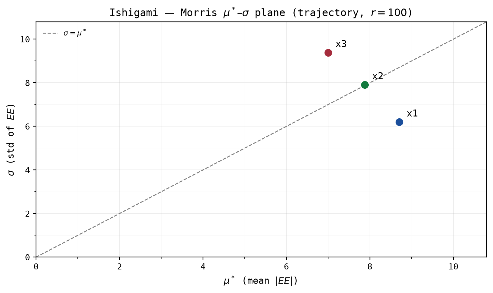
The screening verdict here is that no input can be dropped. That is a real answer, and it cost 63 runs.

The grid resolution is a real choice

num_levels sets the grid the trajectory design walks, and the step is delta = p / (2 * (p - 1)) of the unit range. At the default p = 4 that step is two thirds of each input's range. That is a very coarse difference, and on a periodic response it can alias.

Ishigami shows this in the numbers above. Its x2 term is 7 * sin(x2)^2 on [-pi, pi]. The four grid levels land at -pi, -pi/3, pi/3, pi, where sin^2 takes the values 0, 3/4, 3/4, 0, and a two-level step always connects a 0 to a 3/4. Every elementary effect of x2 therefore has magnitude exactly 7 * 0.75 / (2/3) = 7.875. Not approximately. Exactly.

for p in (4, 8, 20):
    sr = jaxgsa.morris.sample(PROBLEM, n_trajectories=50, num_levels=p, seed=42, verbose=False)
    r = jaxgsa.morris.analyze(sr, evaluate(jnp.asarray(sr.samples)), verbose=False)
    print(f"num_levels={p:2d}  n_runs={sr.n_runs:3d}  mu_star={r.mu_star}  sigma={r.sigma}")

num_levels= 4  n_runs= 63  mu_star=[8.453911 7.875    7.498556]  sigma=[6.266625  7.9485855 9.765831 ]
num_levels= 8  n_runs=169  mu_star=[9.295623  3.3047838 6.264612 ]  sigma=[11.627379  3.463286  8.936818]
num_levels=20  n_runs=196  mu_star=[9.278381  1.3413888 5.7308774]  sigma=[10.888729   1.4947498  8.25101  ]

x2's mu_star falls from 7.88 to 1.34 as the grid gets finer, and its rank drops from second to third. Nothing warns you about this, because nothing is wrong. A Morris measure is defined relative to the step the design takes, and a two-thirds-of-range step on a bumpy function is a legitimate but very blunt instrument. The failure mode to watch for is a mu_star that moves a lot when you change num_levels, and its tell is a suspiciously round or repeated value. If your model is oscillatory in an input, raise num_levels or switch to the radial design below, which uses random step sizes and cannot alias in this way.

How many trajectories are enough

Trajectories are generated in order, so the first m of an r-trajectory design are exactly the design you would have got by asking for m directly at the same seed. Sample once at the largest r you can afford and slice down. No re-evaluation.

sr_full = jaxgsa.morris.sample(PROBLEM, n_trajectories=200, seed=42, verbose=False)
Y_full = evaluate(jnp.asarray(sr_full.samples))
print("n_runs at r=200:", sr_full.n_runs)

for r in (10, 25, 50, 100, 200):
    s, y = sr_full.downsample(r, Y_full)
    out = jaxgsa.morris.analyze(s, y, verbose=False)
    order = [PROBLEM.names[i] for i in (-out.mu_star).argsort()]
    print(f"r={r:3d}  n_runs={s.n_runs:4d}  mu_star={out.mu_star}  order={order}")

n_runs at r=200: 64
r= 10  n_runs=  31  mu_star=[11.453334   7.875001   6.2487984]  order=['x1', 'x2', 'x3']
r= 25  n_runs=  53  mu_star=[9.953622  7.8750005 5.9988456]  order=['x1', 'x2', 'x3']
r= 50  n_runs=  63  mu_star=[8.453911 7.875    7.498556]  order=['x1', 'x2', 'x3']
r=100  n_runs=  64  mu_star=[8.703863  7.8750005 6.998652 ]  order=['x1', 'x2', 'x3']
r=200  n_runs=  64  mu_star=[8.016495  7.8750005 6.373773 ]  order=['x1', 'x2', 'x3']

The ranking is settled by r = 10, on 31 model runs. The values keep drifting by 10 to 20 percent after that, which is the honest answer to "how many trajectories": you need far fewer for a ranking than for a stable number, and a ranking is all Morris promises. For screening, 10 to 50 trajectories is the usual range. Push higher only if two inputs stay close enough to matter and you need to separate them.

Watch the n_runs column at the same time. It stops at 64 and stays there, because a 4-level grid over 3 inputs has 4^3 = 64 distinct points and by r = 100 the design has visited all of them. Every trajectory after that is free. At r = 100 the accounting is 400 expanded rows down to 64 unique evaluations — duplicates_removed=336 (84.0%), an 84% saving over the nominal r * (D + 1) = 400 runs. That saturation is specific to a coarse grid in low dimension. At D = 10 the grid has a million points and you will never see it.

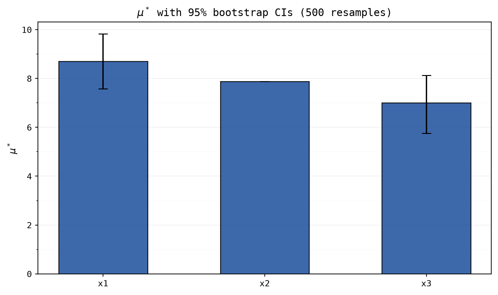
If you want to know whether two inputs are genuinely ordered or just happen to be, bootstrap over trajectories. Pass n_bootstrap and a JAX key.

import jax

sr = jaxgsa.morris.sample(PROBLEM, n_trajectories=50, seed=42, verbose=False)
Y = evaluate(jnp.asarray(sr.samples))

res = jaxgsa.morris.analyze(sr, Y, n_bootstrap=500, key=jax.random.key(0), verbose=False)
print("mu_star     :", res.mu_star)
print("mu_star_conf:", res.mu_star_conf)

mu_star     : [8.453911 7.875    7.498556]
mu_star_conf: [[ 6.7042475  7.875      5.748894 ]
 [10.203573   7.8750005  9.24822  ]]

Row 0 is the lower bound of each mu_star and row 1 the upper. All three intervals overlap, so this run does not separate the three inputs, which agrees with the drift you saw in the r sweep.

The interval on x2 is [7.875, 7.875], a single point. Read that as an alarm, not as precision. The bootstrap resamples trajectories, and every trajectory gives x2 the identical elementary-effect magnitude for the grid reason above, so no resample can produce a different mean. A zero-width Morris interval means the design is not resolving the input, not that the design has nailed it.

A cheap convergence check

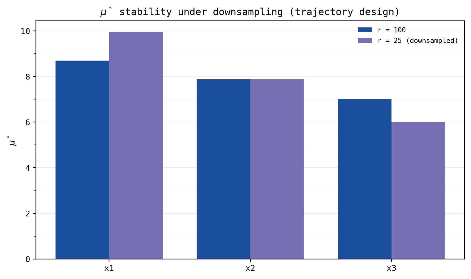
Sample once at the largest r, then confirm the ranking survives a smaller one. The script samples at r = 100 and downsamples to 25 trajectories:

import numpy as np
import jax.numpy as jnp

sr = jaxgsa.morris.sample(PROBLEM, n_trajectories=100, seed=42, verbose=False)
Y = evaluate(jnp.asarray(sr.samples))
result = jaxgsa.morris.analyze(sr, Y, verbose=False)

sr_25, Y_25 = sr.downsample(25, np.asarray(Y))
result_25 = jaxgsa.morris.analyze(sr_25, jnp.asarray(Y_25), verbose=False)


def ranking(mu_star):
    return " > ".join(PROBLEM.names[i] for i in np.argsort(-np.asarray(mu_star)))


print(f"r=100 ranking: {ranking(result.mu_star)}   ({sr.n_runs} unique evals)")
print(f"r=25  ranking: {ranking(result_25.mu_star)}   ({sr_25.n_runs} unique evals)")
print(f"rankings stable: {ranking(result.mu_star) == ranking(result_25.mu_star)}")

r=100 ranking: x1 > x2 > x3   (64 unique evals)
r=25  ranking: x1 > x2 > x3   (53 unique evals)
rankings stable: True

A quarter of the trajectories still yields 53 unique evaluations, and the ranking does not move. rankings stable: True is a cheap gate to put in front of the expensive part of a screening pipeline.

Radial design

method="radial" (Campolongo et al. 2011) replaces the grid walk with star designs around scrambled-Sobol' base points. Each star moves out from its base point along one input at a time, so the structure is the same, but the step length is whatever the quasi-random draw gives instead of a fixed grid stride.

sr_radial = jaxgsa.morris.sample(PROBLEM, n_trajectories=50, method="radial", seed=42)
r_radial = jaxgsa.morris.analyze(sr_radial, evaluate(jnp.asarray(sr_radial.samples)), verbose=False)
print("radial mu_star:", r_radial.mu_star, "sigma:", r_radial.sigma)

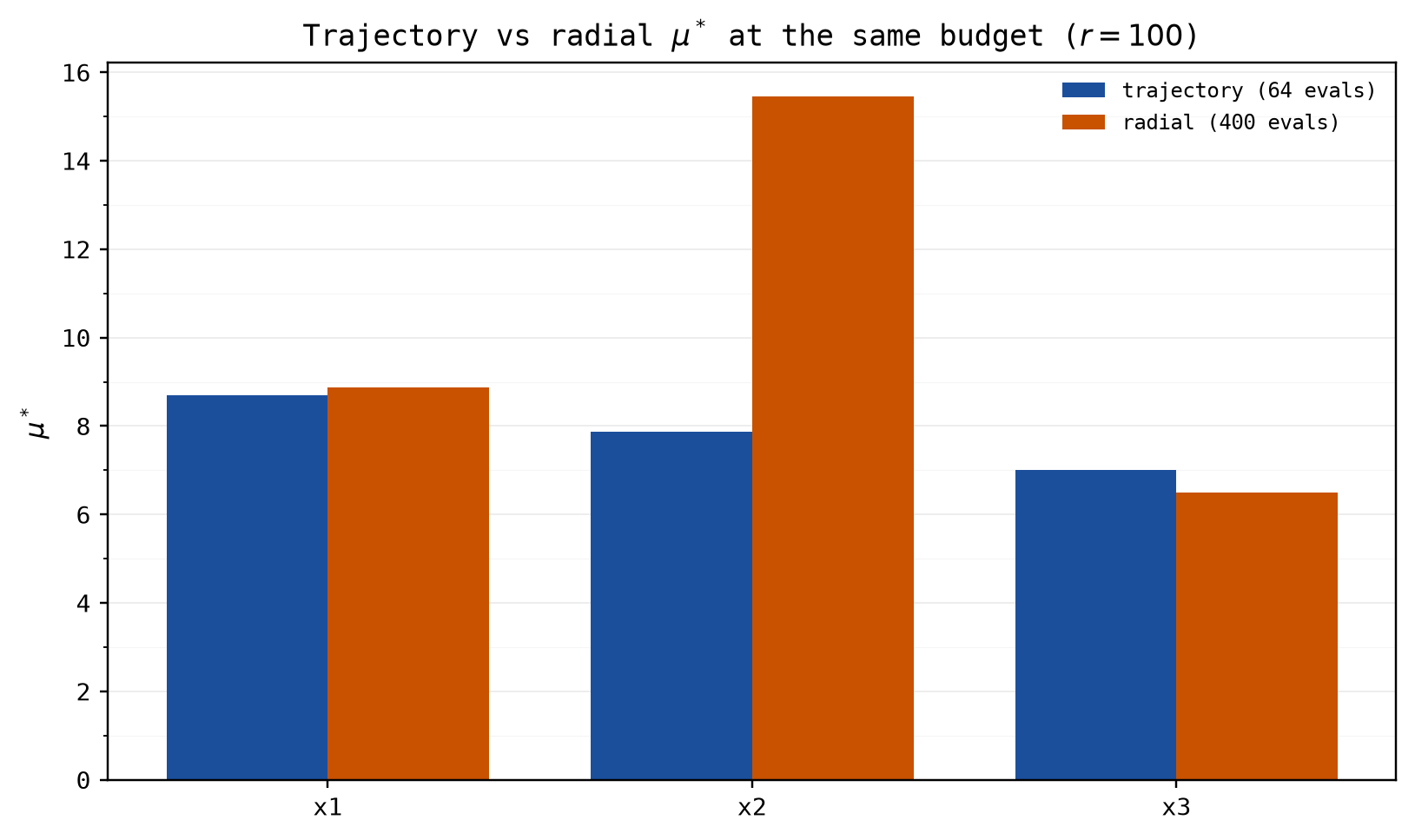
jaxgsa.morris.sample: D=3, method=radial, n_trajectories=50, n_expanded=200, n_runs=200, duplicates_removed=0 (0.0%)
radial mu_star: [ 9.780813  14.439876   6.5912347] sigma: [15.838157 19.575945 11.882108]

Two things changed. The deduplication is gone: 200 rows in, 200 rows out, so the radial design costs the full r * (D + 1) where the grid design did not. And x2 now reads 14.4 rather than 7.9, because the random step sizes sample the whole shape of 7 * sin(x2)^2 instead of the two grid values it happened to connect. Radial steps can also land on the steep local slopes the grid never visits. The derivative of 7 * sin(x2)^2 is 7 * sin(2*x2), with magnitude up to 7 where the response is steepest. The fixed delta = 2/3 grid step always connects the same two sampled values, so it reports one secant slope with the steep parts averaged away. The radial number is the trustworthy one here. num_levels is ignored by this design, and scramble=True (the default) should stay on.

Morris measures from a Saltelli design, for free

If you have already paid for a Sobol run, you can read Morris measures off the same evaluations without a single extra model call. A Saltelli design holds two independent matrices A and B, plus one matrix AB_j per input in which column j of A is swapped for column j of B. Inside one base point, A and AB_j differ in exactly one input. That is a radial star, so SobolSamples.to_morris() just relabels the design.

samples = jaxgsa.sobol.sample(PROBLEM, 0, base_n=512, seed=0)
Y = evaluate(jnp.asarray(samples.samples))

sobol_result = jaxgsa.sobol.analyze(samples, Y)
morris_result = jaxgsa.morris.analyze(samples.to_morris(), Y)

print("ST     :", sobol_result.ST)
print("mu_star:", morris_result.mu_star)

jaxgsa.sobol.sample: D=3, mode=second-order, base_n=512, requested_runs>=4096, n_runs=4096, n_expanded=4096, duplicates_removed=0 (0.0%), scramble=True
jaxgsa.sobol.analyze
  problem: D=3 (x1, x2, x3)
    marginals: uniform=3
    correlation: independent
    output: N=4096 runs, T=1 x K=1 output slice
    invalid: none found in 512 Saltelli groups (policy 'raise')
  timing:
    estimators (includes compile on the first call): 0.9145 s
    slice_chunk_size: 1 (resolved from the memory budget)
    estimator: saltelli-jansen
  results: top 3 of 3 parameters by ST
    1. x1  ST=0.4527
    2. x2  ST=0.4429
    3. x3  ST=0.2546
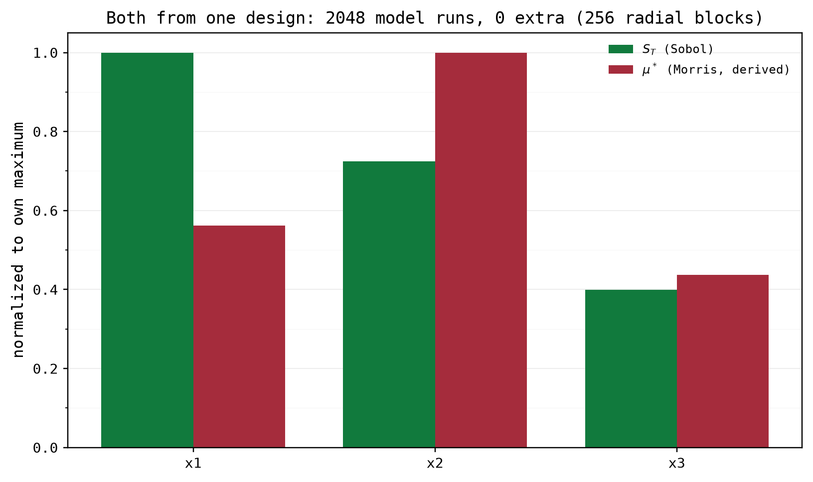
jaxgsa.sobol.SobolSamples.to_morris: D=3, mode=second-order, base_n=512, blocks=512, effects=1536, reusing n_runs=4096 existing evaluations (0 new model runs)
jaxgsa.morris.analyze
  problem: D=3 (x1, x2, x3)
    marginals: uniform=3
    correlation: independent
    output: N=2048 runs, T=1 x K=1 output slice
    invalid: none found in 512 trajectories (policy 'raise')
  timing:
    estimator (includes compile on the first call): 0.2207 s
  results: top 3 of 3 parameters by mu_star
    1. x2  mu_star=14.94
    2. x1  mu_star=8.611
    3. x3  mu_star=6.617
ST     : [0.45272487 0.442889   0.25457737]
mu_star: [ 8.610636  14.939382   6.6169825]

to_morris prints its own accounting line, and the phrase to check is 0 new model runs. The same Y array feeds both analyses.

Compare the two rankings, and notice that they disagree. ST puts x1 first at 0.453 with x2 just behind at 0.443. mu_star puts x2 first at 14.9, well clear of x1 at 8.6. Neither is wrong. ST is a variance fraction and mu_star is a mean absolute slope on the model's own scale, and the two weight a sharply peaked response differently. This is the reason to treat Morris as a screen. Both agree that x3 is last and that nothing is negligible, and that is the decision Morris was asked to make.

The two measures are two weightings of the same increments. Jansen's total-order estimator is $E[{\mathrm{\Delta }}_j^{2}E{E}_j^2]/(2\cdot \mathrm{Var}Y)$ — with ${\mathrm{\Delta }}_j$ the input step and $E{E}_j$ the elementary effect, the product is just the squared output change — while Morris reports ${\mu }^{\ast }=E|E{E}_j|$. Same increments, weighted differently: Jansen weights each by its square, Morris by its absolute value, and that is why the ranking can shift.

Screening verdicts are design-dependent: when in doubt, keep every parameter that either design flags as important.

Because the two results come from the same model outputs, they are not independent of each other. Agreement between mu_star and ST here is not a validation of either.

to_morris() returns an ordinary MorrisSamples with method="radial", so bootstrap intervals, multi-output shapes, to_dataset(), downsample() and save() all work on it. n_trajectories equals base_n, one radial block per base point. A second-order design also carries a block based at B, but for additive contributions that block measures the same effect, so harvesting it would double the apparent sample size and narrow bootstrap intervals without adding information. It is deliberately left unused.

Multi-output example

Return every quantity you might want in one array. Extra outputs cost no extra model runs. Y of shape (n_runs, K) gives measures of shape (K, D), and (n_runs, T, K) gives (T, K, D).

import jax.numpy as jnp
import jaxgsa

problem = jaxgsa.Problem.from_dict(
    {"amplitude": (0.5, 2.0), "frequency": (1.0, 5.0), "damping": (0.01, 0.5)},
    output_names=("displacement", "velocity"),
)


def multi_output_model(X):
    amp, freq, damping = X[:, 0], X[:, 1], X[:, 2]
    return jnp.stack(
        [
            amp * jnp.sin(freq) * jnp.exp(-damping),
            amp * jnp.cos(freq) * jnp.exp(-damping),
        ],
        axis=-1,
    )


sr = jaxgsa.morris.sample(problem, n_trajectories=50, seed=42)
Y = multi_output_model(jnp.asarray(sr.samples))
result = jaxgsa.morris.analyze(sr, Y)
print("mu_star:\n", result.mu_star)

jaxgsa.morris.sample: D=3, method=trajectory, n_trajectories=50, num_levels=4, n_expanded=200, n_runs=63, duplicates_removed=137 (68.5%)
jaxgsa.morris.analyze
  problem: D=3 (amplitude, frequency, damping)
    marginals: uniform=3
    correlation: independent
    output: N=200 runs, T=1 x K=2 output slices
    invalid: none found in 50 trajectories (policy 'raise')
  timing:
    estimator (includes compile on the first call): 0.2276 s
  results: top 3 of 3 parameters by mu_star, mean over 2 output slices
    1. frequency  mu_star=1.904
    2. amplitude  mu_star=0.7952
    3. damping    mu_star=0.3143
mu_star:
 [[0.8995233  2.1025996  0.3571391 ]
 [0.6908595  1.7062234  0.27144668]]

Row 0 is displacement and row 1 is velocity, following output_names. So result.mu_star[1, 0] is the importance of amplitude for velocity. The top-k table in the summary averages over output slices, which is a convenience for a quick look; when the outputs have different magnitudes, read the array rows separately or pass standardize_outputs=True so each slice is expressed in units of its own standard deviation.

xarray export

MorrisResult.to_dataset() gives you a labeled xarray.Dataset, so you select by parameter and output name instead of counting axes. This picks up the result from the multi-output example above.

ds = result.to_dataset()
print(ds)
print(ds.mu_star.sel(param="amplitude").values, ds.attrs["space"])

<xarray.Dataset> Size: 276B
Dimensions:  (output: 2, param: 3)
Coordinates:
  * output   (output) <U12 96B 'displacement' 'velocity'
  * param    (param) <U9 108B 'amplitude' 'frequency' 'damping'
Data variables:
    mu       (output, param) float32 24B -0.08051 -2.103 ... -0.4799 0.05442
    mu_star  (output, param) float32 24B 0.8995 2.103 0.3571 0.6909 1.706 0.2714
    sigma    (output, param) float32 24B 0.9521 1.036 0.396 0.7309 1.901 0.3022
Attributes:
    space:    unit
[0.8995233 0.6908595] unit

The space attribute travels with the data, so a dataset written to disk still says which coordinate system its numbers are in. For time-series results pass time_coords to label the time axis. With a bootstrap the dataset also carries mu_lower, mu_upper, mu_star_lower, and the rest.

Gaussian inputs

The Morris design deliberately touches the unit-cube boundaries, and an unbounded inverse CDF sends 0 and 1 to infinity. Each open side of a Gaussian marginal is therefore pulled in by truncation_quantile (default 1e-4, so the grid probes the 0.01% to 99.99% range) before the transform. A side you bounded yourself with an explicit low or high is left exactly where you put it, so a two-sided truncated Gaussian is sampled as declared. Uniform marginals are untouched.

problem = jaxgsa.Problem.from_dict(
    {
        "x1": (-1.0, 1.0),
        "x2": {"dist": "gaussian", "mean": 0.0, "variance": 1.0},
    }
)

sr = jaxgsa.morris.sample(problem, n_trajectories=50, seed=42)
X = jnp.asarray(sr.samples)
Y = X[:, 0] + X[:, 1] ** 2

result = jaxgsa.morris.analyze(sr, Y)
print("mu_star:", result.mu_star)

jaxgsa.morris.sample: D=2, method=trajectory, n_trajectories=50, num_levels=4, n_expanded=150, n_runs=16, duplicates_removed=134 (89.3%)
jaxgsa.morris.analyze
  problem: D=2 (x1, x2)
    marginals: uniform=1, gaussian=1
    correlation: independent
    output: N=150 runs, T=1 x K=1 output slice
    invalid: none found in 50 trajectories (policy 'raise')
  timing:
    estimator (includes compile on the first call): 0.1468 s
  results: top 2 of 2 parameters by mu_star
    1. x2  mu_star=20.47
    2. x1  mu_star=2
mu_star: [ 2.       20.472542]

Sixteen model runs for a two-input screen, because a 4-level grid over 2 inputs has 16 points.

On an unbounded marginal mu_star has no limit as the truncation shrinks. The design always includes unit levels 0 and 1 exactly, so a smaller truncation_quantile reaches further into the tail and the effects grow with it. The 20.47 above is a number about this truncation setting as much as about the model. Rankings survive the choice; magnitudes do not. If you need magnitudes comparable across methods, fix one bounded input model up front:

bounded = jaxgsa.Problem.from_dict(
    {
        "x1": (-1.0, 1.0),
        "x2": {"dist": "gaussian", "mean": 0.0, "variance": 1.0},
    },
    truncate_gaussians=1e-4,
)
print(bounded.input_specs[1])

GaussianSpec(mean=0.0, variance=1.0, low=-3.7190164854556804, high=3.7190164854557084)

That writes explicit low and high into every Gaussian that does not already declare them, at that marginal's own q and 1 - q quantiles, and every method then sees the same problem.

Physical units

Elementary effects are computed in unit-cube coordinates. That is what makes mu_star comparable across inputs whose physical ranges differ by orders of magnitude. to_physical_units() returns a copy with each measure divided by its input's high - low, which puts them on the derivative scale that DGSM reports.

import jax.numpy as jnp
import jaxgsa
from jaxgsa.benchmarks.ishigami import PROBLEM, evaluate

sr = jaxgsa.morris.sample(PROBLEM, n_trajectories=50, seed=42, verbose=False)
result = jaxgsa.morris.analyze(sr, evaluate(jnp.asarray(sr.samples)), verbose=False)

physical = result.to_physical_units()
print("space:", result.space, "->", physical.space)
print("unit     mu_star:", result.mu_star)
print("physical mu_star:", physical.mu_star)

space: unit -> physical
unit     mu_star: [8.453911 7.875    7.498556]
physical mu_star: [1.3454816 1.2533451 1.1934322]

The original result is untouched and still reports space == "unit". Ishigami gives all three inputs the same [-pi, pi] range, so the ranking survives; when ranges differ the ranking can and should change, and which one you want depends on whether you are asking "which input should I study" (unit) or "how much does the output move per physical unit of input" (physical).

Calling to_physical_units() twice raises. So does calling it on a problem with a Gaussian marginal, because the inverse-CDF transform is nonlinear and there is no single range to divide by:

ValueError: to_physical_units requires a problem with finite uniform bounds

Shape rules

• (n_runs,) is scalar output.
• (n_runs, K) is K output variables with no time dimension.
• (n_runs, T, K) is T time steps and K outputs.
• Without problem.output_names, a 2D array is always read as (n_runs, K).
• With exactly one name in problem.output_names, a 2D array is read as (n_runs, T), the timepoints of that single output, and flows through as (n_runs, T, 1). A pre-reshaped (n_runs, T, 1) array works too.

Y shape	mu / mu_star / sigma shape
(n_runs,)	(D,)
(n_runs, K)	(K, D)
(n_runs, T, K)	(T, K, D)

D is always the last axis.

Practical caveats

• Evaluate Y on sr.samples, the unique rows. jaxgsa.morris.analyze() rebuilds the expanded trajectory layout itself.
• Morris does not produce Sobol indices. mu_star ranks like ST but is not a variance fraction, and sigma flags interaction without saying with whom.
• An even num_levels (default 4) makes all grid levels equally probable. An odd value warns, because the step then lands off-grid.
• truncation_quantile must lie in (0, 0.5) or sample() raises.
• A trajectory holding any non-finite output raises by default. Pass on_invalid="drop" to remove it. The unit is the whole trajectory block, because an elementary effect is a difference between neighbouring rows inside it and a gap would invent an effect nobody measured. Under 2 surviving trajectories raises; under 10 warns.
• jaxgsa.morris.sample() refuses a Problem with categorical inputs. The design steps each input along a grid, and unordered level codes have no grid. It also refuses a problem with a declared correlation, because the one-at-a-time step assumes it can move one input while the others hold still.
• A design derived through SobolSamples.to_morris() is a radial design, and it estimates E|f(A with B_j) - f(A)| / |B_j - A_j| rather than a fixed-step grid quantity. Compare it against morris.sample(..., method="radial"), not against the default trajectory design. On Ishigami at r=8192 the derived mu_star is [8.68, 15.01, 6.62] against [8.69, 15.02, 6.64] for native radial and [7.59, 7.88, 6.39] for native trajectory.
• Derived blocks whose step is too small to measure are dropped with a warning. At the default scramble=True this does not bite: 0 of 65536 blocks were dropped across 8 seeds at D=3. With scramble=False the drop rate is 21.9% at base_n=64, 9.4% at 256, 2.3% at 1024, and 1.2% at 4096, and the survivors are a biased subsequence. At base_n=64 that reads mu_star for x3 16% low. Keep scramble=True.

See also

• Basic example for the Sobol workflow, the natural next step once screening has told you which inputs deserve it.
• DGSM for the autodiff version of the same idea, with a provable bound on ST attached.
• eFAST for frequency-based variance decomposition.
• xarray labeled output for named access by parameter, output and time.
• Methods for the theory and the method comparison.
• API reference for every parameter.