Batch reactor

This example answers one question about a chemical reactor: of its three operating conditions, which one drives the spread in outlet concentration, and does the answer change during the batch. The output is a ranked set of Sobol indices with error bars, plus a plot of how that ranking moves in time. A Sobol index is the share of output variance attributed to one input.

The reactor runs a first-order liquid-phase reaction $A\to B$. Three inputs vary: the inlet concentration $C_{A,0}$, the temperature $T$, and the $\mathrm{pH}$. The rate constant $k(T,\mathrm{pH})$ combines an Arrhenius temperature dependence with a Hill-type pH saturation curve. The inlet concentration $C_{A,0}$ feeds the mass balance directly. Starting from an empty reactor, the mass balance has a closed-form solution, so the model is a formula rather than an integrator and every point costs almost nothing to evaluate.

The mechanistic model is treated as already fitted. The question is variance attribution across the operating envelope, not parameter estimation.

The full script lives at examples/batch_reactor_gsa.py. Run it with uv run python examples/batch_reactor_gsa.py; it prints the transcripts below and draws the three plots discussed at the end.

What the run prints

The script form prints the sampler line, the output shape, and the verbose analysis summary that analyze emits by default in 1.0:

jaxgsa.sobol.sample: D=3, mode=second-order, base_n=512, requested_runs>=4096, n_runs=4096, n_expanded=4096, duplicates_removed=0 (0.0%), scramble=True
unique Saltelli rows: (4096, 3)
output shape: (4096, 40, 1)  (N, T, K)
jaxgsa.sobol.analyze
  problem: D=3 (Ca0, temperature_C, pH)
    marginals: uniform=3
    correlation: independent
    output: N=4096 runs, T=40 x K=1 output slices
    invalid: none found in 512 Saltelli groups (policy 'raise')
  timing:
    estimators (includes compile on the first call): 1.395 s
    slice_chunk_size: 40 (resolved from the memory budget)
    bootstrap slice_chunk_size: 40 (resolved from the memory budget)
    estimator: saltelli-jansen
  results: top 3 of 3 parameters by ST, mean over 40 output slices
    1. Ca0            ST=0.6291  [0.564, 0.7124]
    2. pH             ST=0.2279  [0.206, 0.2583]
    3. temperature_C  ST=0.156  [0.1354, 0.1796]
SobolResult(S1=(40, 1, 3), S1_conf=(2, 40, 1, 3), ST=(40, 1, 3), ST_conf=(2, 40, 1, 3), S2=(40, 1, 3, 3), S2_conf=(2, 40, 1, 3, 3), estimator='saltelli-jansen', ci=CIInfo(level=0.95, method='quantile', n_bootstrap=200, replicates=None))

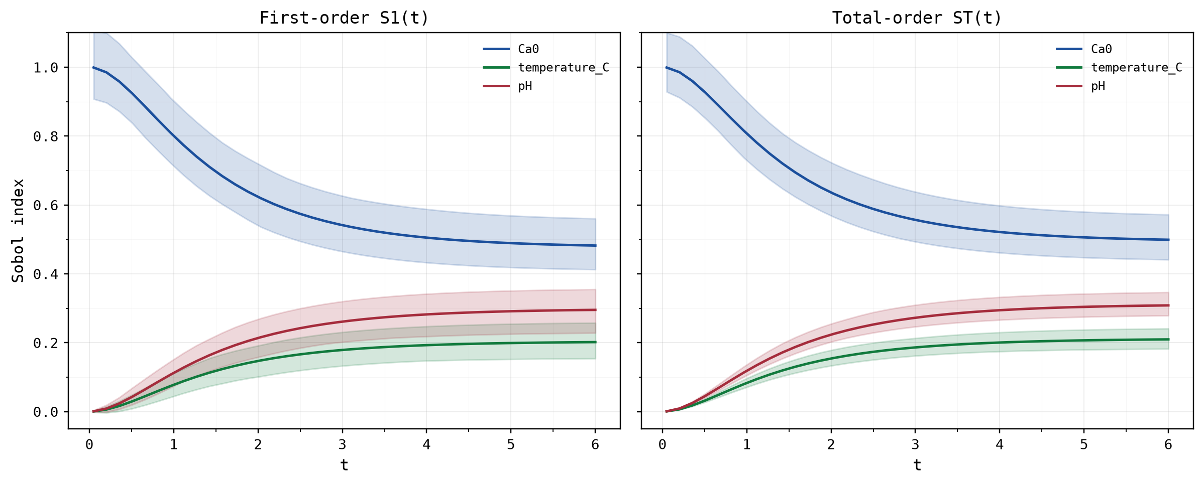
Read that ranking with care. The line says mean over 40 output slices, because the output is a trajectory and there are 40 sets of indices, one per time step. The summary averages them so it has something to rank. A mean over time is a summary, not the answer, and on this model the answer changes completely between the first time step and the last. That is what the time-resolved plot in the script is for.

The numbers behind the plots

Here is the script's analysis as a self-contained block, with the two time steps that matter printed out.

import jax
import jax.numpy as jnp
import numpy as np

import jaxgsa

T_REF, R_GAS, EA = 298.15, 8.314e-3, 30.0
K_BASELINE, K_AMPLITUDE, PH50, HILL, TAU = 0.14, 1.05, 5.85, 5.0, 2.0


def k_rate(temperature_C, pH):
    T_K = temperature_C + 273.15
    arrhenius = jnp.exp(-EA / R_GAS * (1.0 / T_K - 1.0 / T_REF))
    return (K_BASELINE + K_AMPLITUDE / (1.0 + (pH / PH50) ** HILL)) * arrhenius


def trajectory(Ca0, temperature_C, pH, ts):
    k = k_rate(temperature_C, pH)
    return Ca0 / (1.0 + k * TAU) * (1.0 - jnp.exp(-(1.0 / TAU + k) * ts))


problem = jaxgsa.Problem.from_dict(
    {"Ca0": (0.75, 1.5), "temperature_C": (15.0, 35.0), "pH": (4.5, 7.5)},
    output_names=("Ca",),
)
design = jaxgsa.sobol.sample(problem, n_samples=4096, seed=0, calc_second_order=True)

ts = jnp.asarray(np.linspace(0.05, 6.0, 40))
X = jnp.asarray(design.samples)
Y = trajectory(X[:, 0:1], X[:, 1:2], X[:, 2:3], ts[None, :])[..., None]
print("output shape:", Y.shape, " (N, T, K)")

result = jaxgsa.sobol.analyze(design, Y, n_bootstrap=200, key=jax.random.key(0))

S1 = np.asarray(result.S1)[:, 0, :]
ST = np.asarray(result.ST)[:, 0, :]
S2 = np.asarray(result.S2)[:, 0, :, :]

for label, t in (("t = 0.05 (start-up)", 0), ("t = 6.0 (steady state)", 39)):
    print(f"\n{label}")
    for i, name in enumerate(problem.names):
        print(f"  {name:<14} S1={S1[t, i]:.4f}  ST={ST[t, i]:.4f}")

print("\npairwise S2 at t = 6.0")
for i in range(3):
    for j in range(i + 1, 3):
        print(f"  {problem.names[i]}/{problem.names[j]}: {S2[39, i, j]:.4f}")

It reprints the two verbose blocks shown above, then:

t = 0.05 (start-up)
  Ca0            S1=0.9991  ST=0.9990
  temperature_C  S1=0.0004  ST=0.0004
  pH             S1=0.0007  ST=0.0006

t = 6.0 (steady state)
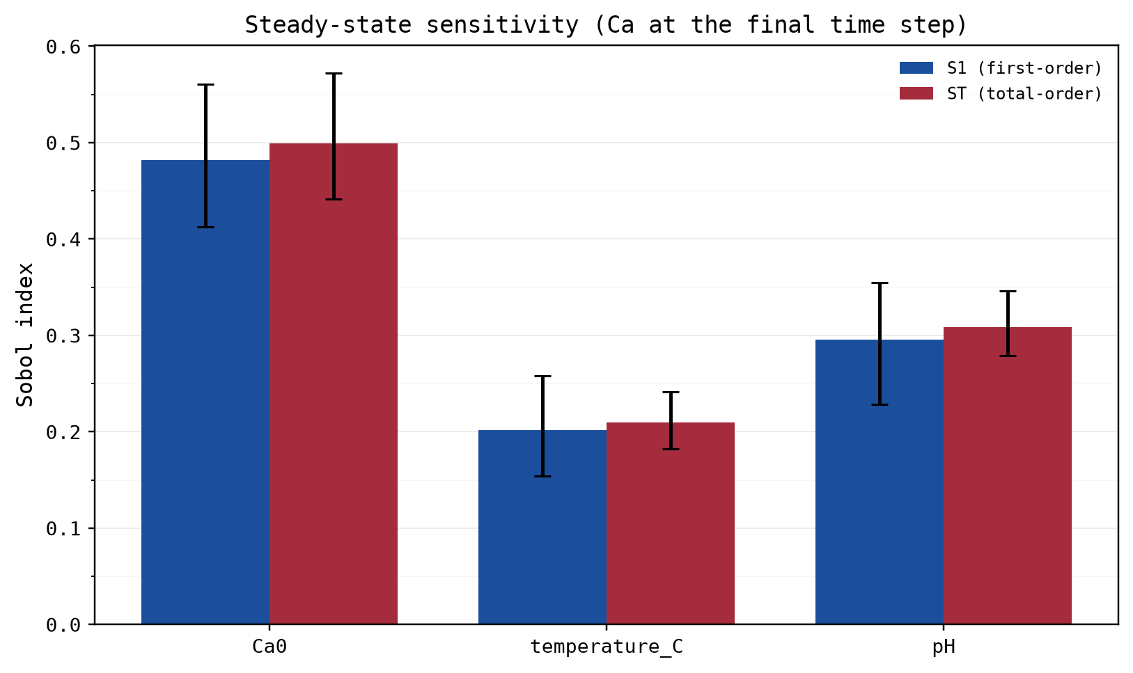
  Ca0            S1=0.4821  ST=0.4990
  temperature_C  S1=0.2016  ST=0.2096
  pH             S1=0.2952  ST=0.3083

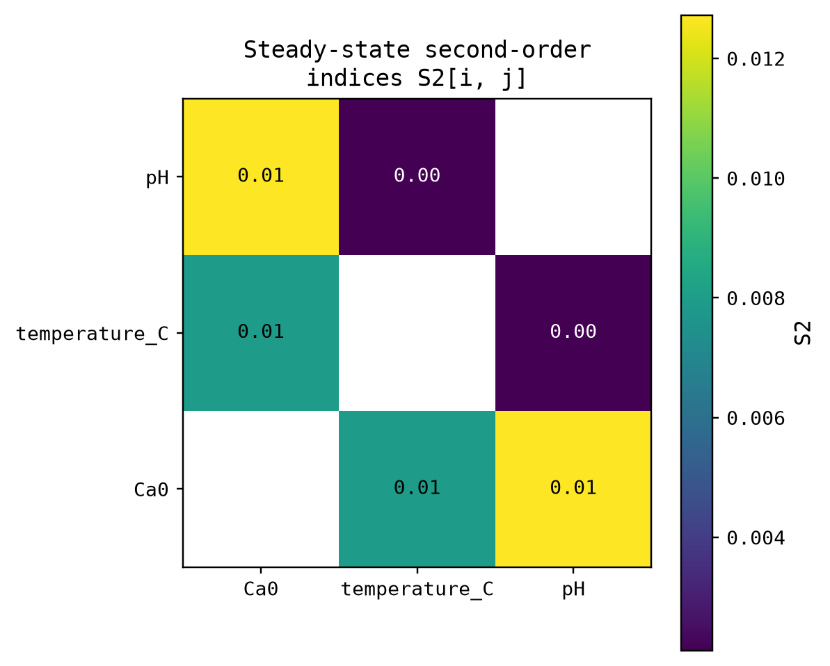
pairwise S2 at t = 6.0
  Ca0/temperature_C: 0.0081
  Ca0/pH: 0.0125
  temperature_C/pH: 0.0000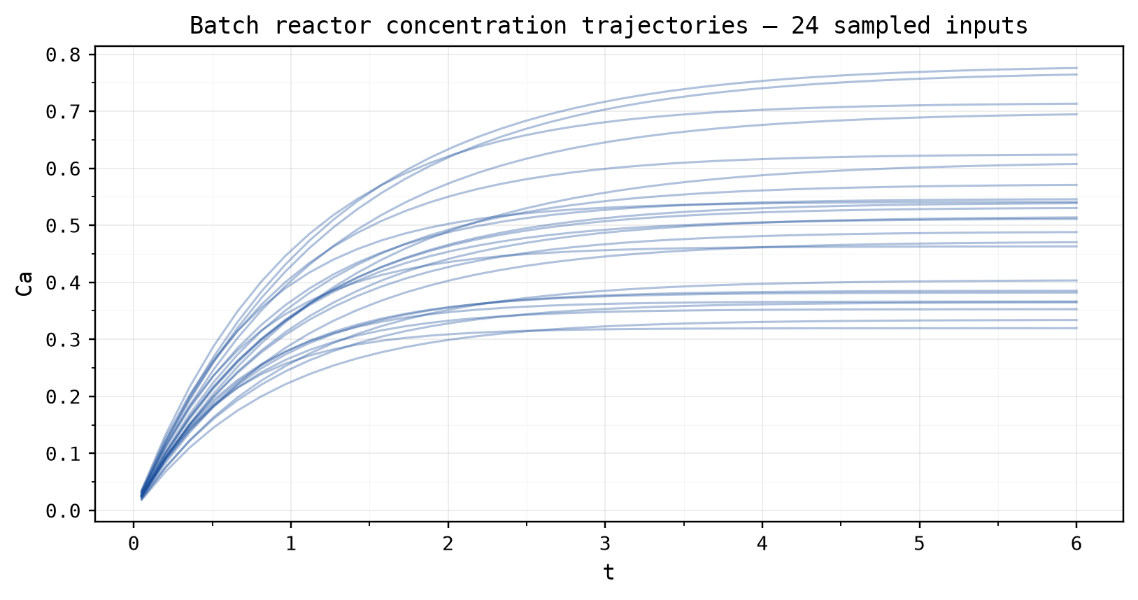

Three things fall out of that.

At the first time step, $C_{A,0}$ explains 99.9% of the variance and the kinetics explain nothing. The reaction has not had time to act, so the concentration is still filling towards its asymptote and scales with whatever you fed in. A one-time-step sensitivity study of this reactor would conclude that temperature and pH do not matter, which is wrong by the end of the batch.

By steady state, the split is roughly 50/30/20 between $C_{A,0}$, $\mathrm{pH}$ and $T$. $\mathrm{pH}$ overtakes $T$ because the Hill curve is steep near ${\mathrm{pH}}_{50}=5.85$ and the sampled range $[4.5,7.5]$ crosses it, while the 20 K temperature range moves the Arrhenius factor by about a factor of two. Ranges drive rankings. Widen the temperature box and the ordering flips.

The interactions are all small. At steady state $S_T$ exceeds $S_1$ by 0.008 for $T$, 0.013 for $\mathrm{pH}$ and 0.017 for $C_{A,0}$, and the largest pairwise index is 0.0125 for $C_{A,0}$ with $\mathrm{pH}$. Temperature and pH register 0.0000 together at steady state, despite entering the model only through the product $k(T,\mathrm{pH})$, which is a good reminder that "these two appear in the same term" is not the same claim as "these two interact in the variance sense". The response is close to additive across the operating box.

Why these settings

n_samples=4096 gives base_n=512, and with calc_second_order=True the design costs base_n * (2D + 2) = 4,096 model runs. That is generous for three inputs, and the reason is the second-order indices. $S_2$ is a difference of variance estimates and it is much noisier than $S_1$, so it needs the extra budget to come out stable at three decimal places. Drop calc_second_order and the same accuracy on $S_1$ and $S_T$ costs base_n * (D + 2) instead.

n_bootstrap=200 and key=jax.random.key(0) fill every _conf array. 200 resamples is at the low end. It is enough for error bars you plot, and if you want to quote endpoints to three decimals, raise it. The resamples reuse the outputs you already have, so raising it costs no model runs. See bootstrap confidence intervals.

The output is (4096, 40, 1): 4,096 runs, 40 time steps, one output. jaxgsa computes an independent set of indices for every (t, k) slice, so S1 comes back as (40, 1, 3) and S2 as (40, 1, 3, 3). The trailing 1 is the output axis, and keeping it means the plotting code does not need a special case for the single-output run. See multi-output and time-series.

What the script draws

Running the script produces three figures. The steady-state bar chart shows $S_1$ and $S_T$ at the final time step with the bootstrap 95 % confidence intervals as error bars.

The time-resolved plot traces $S_1(t)$ and $S_T(t)$ for each input with the bootstrap envelopes shaded — it is where the ranking change described above becomes visible as two curves crossing.

The pairwise $S_{ij}$ heatmap at the final time step rounds it out.

See also

• Bootstrap confidence intervals for what the error bars in these plots cover.
• Multi-output and time-series for the (N, T, K) shape rules used here.
• Save and reload a design for running the 4,096 evaluations somewhere other than your laptop.