DGSM (derivative-based global sensitivity measures)

DGSM averages the model's partial derivatives over the input distribution and turns those averages into two numbers that frame each input's total Sobol index ST. It does not compute ST, and for most inputs it does not need to, because the question is usually "can I fix this one" rather than "what exactly is its share".

The two measures it works from are

• nu_i = E[(df/dx_i)^2], the mean squared partial derivative. This is the ranking measure.
• sigma_i = E[df/dx_i], the mean signed derivative.

and the two expressions built from them are

• upper_bound_i = C_i * nu_i / Var(Y). This is the Poincare inequality, and it is a genuine bound: ST_i is never above it. C_i is the Poincare constant of input i's own marginal, the smallest factor for which Var(g(X_i)) <= C_i * E[g'(X_i)^2] holds for every smooth g.
• lower_bound_i = Var(x_i) * sigma_i^2 / Var(Y). Kucherenko & Song (2016) prove this is a lower bound on ST_i when input i's marginal is an untruncated Gaussian. Under a uniform or truncated marginal it is an estimate: it equals ST_i when the response is linear in that input and it degrades gracefully near linearity, but it is not safe as a floor for a strongly curved response. There is a worked counter-example further down.

The upper bound is what makes DGSM more than a ranking heuristic. An input whose upper bound comes back at 1e-7 cannot be responsible for more than a ten-millionth of the output variance, and no amount of extra sampling will change that. It is a proof, not an estimate that happened to be small.

The cost is one autodiff sweep over a plain Monte Carlo sample. No structured design, no sample() function, and no fixed relationship between the sample size and D. The example below settles three of four inputs on 500 model runs where the equivalent Sobol design needed 40960.

The full script is examples/dgsm_benchmark.py, run with uv run python examples/dgsm_benchmark.py.

Import style

from jaxgsa import dgsm
# dgsm.analyze(...)

monte_carlo lives in jaxgsa.sampling, not in jaxgsa.dgsm. Call it as jaxgsa.sampling.monte_carlo().

fn takes one row, not a batch

Every other method in this package calls your model on the whole (N, D) matrix. DGSM does not. fn maps one row of shape (D,) to (), (K,), or (T, K), because that is the signature JAX differentiates. analyze does the vectorizing and the batching itself.

If you hand it a batch model, it says so before running anything. The check traces fn on one row with jax.eval_shape, so an expensive model costs nothing to reject:

ValueError: fn could not be evaluated on a single sample row: IndexError: Too many indices: array is 1-dimensional, but 2 were indexed
jaxgsa.dgsm.analyze differentiates a one-sample function: it maps one row of shape (4,) to a scalar (), a (K,) vector, or a (T, K) array. Wrap a batch model that takes (N, D) as `lambda x: model(x[None, :])[0]`.

The wrapper suggestion appears only when the failure looks like a batch callable. Any other trace error is reported on its own terms with no guess at the cause.

Scalar example

A small groundwater head model with four inputs, one of which is a passive tracer concentration that barely enters the output. This is the shape of problem DGSM is for: several inputs, a suspicion that some do not matter, and a model you can differentiate.

import jax.numpy as jnp
import jaxgsa

problem = jaxgsa.Problem.from_dict(
    {
        "inflow": (2.0, 8.0),
        "porosity": (0.1, 0.4),
        "roughness": (0.02, 0.05),
        "tracer": (0.0, 1.0),
    }
)


def head(x):
    """Unbatched: (4,) -> ()."""
    inflow, porosity, roughness, tracer = x
    return inflow / porosity + 40.0 * jnp.sqrt(roughness) + 0.02 * tracer


X = jaxgsa.sampling.monte_carlo(problem, n=20000, seed=0)
result = jaxgsa.dgsm.analyze(problem, head, jnp.asarray(X))

print("upper:", result.upper_bound)
print("lower:", result.lower_bound)
print("var_y:", result.var_y)

jaxgsa.dgsm.analyze
  problem: D=4 (inflow, porosity, roughness, tracer)
    marginals: uniform=4
    correlation: independent
    output: N=20000 runs, T=1 x K=1 output slice
    invalid: none found in 20000 rows (policy 'raise')
  timing:
    model sweep + estimator (includes compile on the first call): 0.5884 s
    gradients: reverse-mode autodiff (T*K=1, D=4)
    batch_size: auto (resolved from the memory budget)
  results: top 4 of 4 parameters by nu
    1. porosity   nu=3.036e+04
    2. roughness  nu=1.224e+04
    3. inflow     nu=24.84
    4. tracer     nu=0.0004
upper: [5.4446208e-01 1.6631646e+00 6.7081735e-03 2.4349364e-07]
lower: [3.8285753e-01 6.9644910e-01 5.4230299e-03 2.0026555e-07]

Read it input by input, because each one gets a different kind of answer.

tracer is bounded above by 2.4e-07. That input is finished. Fix it at any value in its range and the output variance will not notice.

roughness is capped at 0.0067. Not zero, but under one percent of the output variance, which for most purposes is the same decision. The true value is 0.0053, so the cap is only 26% above it. The model is monotone in roughness, and monotone is exactly when the Poincare inequality is nearly an equality.

inflow is capped at 0.544, with a lower estimate of 0.383. Wide, but well away from zero, so the input matters and the only open question is by how much.

porosity has an upper bound of 1.66, which is greater than 1 and therefore says nothing at all. That is the normal outcome for a dominant, strongly nonlinear input, and inflow / porosity on porosity in [0.1, 0.4] is exactly that. Its lower_bound reads 0.696, and this is the one number on the page you should not take at face value. See the next section.

So one call decided three of four inputs. Here is the check against a Sobol run at base_n=65536:

sobol ST: [4.4897085e-01 6.1121655e-01 5.3001028e-03 1.9954255e-07]

Every one of those ST values sits under its DGSM upper bound, and pinning them down this precisely took 655360 model runs against DGSM's 20000.

Where the lower bound stops being a bound

porosity's true ST is 0.6112, which is below its reported lower_bound of 0.696. That is not sampling noise. The Sobol run above agrees with the closed-form answer for this model to four digits.

The literature says exactly when this can happen. Kucherenko & Song (2016) prove ST_i >= Var(x_i) * sigma_i^2 / Var(Y) in their Theorem 6, for a Gaussian input, and nowhere else. The proof runs through Stein's identity, Cov(f, x_i) = E[tau(x_i) * df/dx_i], whose kernel tau is the constant Var(x_i) for an untruncated Gaussian and is not constant for anything else. For U(a, b) it is tau(x) = (x - a)(b - x)/2, which is small near the endpoints and largest in the middle. Replacing it by its mean Var(x_i) is an approximation, not an inequality, and the approximation is what fails here. The paper's lower bounds for uniform inputs, LB1 and LB2, are different quantities that need boundary evaluations and the higher moments E[x_i^m * df/dx_i]. jaxgsa does not compute them. porosity is uniform, so the printed floor carries no proof.

Concretely, Var(x_i) * sigma_i^2 / Var(Y) is exact when f is linear in x_i, because then sigma_i is the slope and the conditional variance is slope^2 * Var(x_i). For a curved response sigma_i is the average slope, and a function that is steep over a small part of its range and flat over the rest has an average slope much larger than its spread justifies. Strip the model down to one input to see it plainly:

problem_1d = jaxgsa.Problem.from_dict({"p": (0.1, 0.4)})
X = jaxgsa.sampling.monte_carlo(problem_1d, n=200000, seed=0)
r = jaxgsa.dgsm.analyze(problem_1d, lambda x: 1.0 / x[0], jnp.asarray(X), verbose=False)
print("lower_bound:", r.lower_bound, " upper_bound:", r.upper_bound)

lower_bound: [1.2888439]  upper_bound: [2.7395327]

With one input the total Sobol index is 1 by definition, and the reported lower bound is 1.289. Any value above 1 is impossible.

So the practical rule is short. Trust upper_bound. The Poincare inequality holds for every marginal jaxgsa supports, and a small upper bound is a proof you can act on. Trust lower_bound as a floor only on a Gaussian input. On a uniform or truncated input, read it as an estimate that is right for a nearly linear response and optimistic for a convex or concave one, and confirm anything that rests on it with Sobol.

What it costs

import numpy as np

for n in (500, 2000, 20000):
    X = jaxgsa.sampling.monte_carlo(problem, n=n, seed=0)
    r = jaxgsa.dgsm.analyze(problem, head, jnp.asarray(X), verbose=False)
    print(f"n={n:6d} upper={np.array2string(np.asarray(r.upper_bound), precision=4)}")

n=   500 upper=[4.7530e-01 1.6285e+00 5.7597e-03 2.1119e-07]
n=  2000 upper=[5.1130e-01 1.6365e+00 6.2901e-03 2.2747e-07]
n= 20000 upper=[5.4446e-01 1.6632e+00 6.7082e-03 2.4349e-07]

Five hundred model runs reach the same verdict as twenty thousand: tracer is provably irrelevant, roughness is tiny, inflow and porosity matter. The second-order Saltelli design for the same four inputs at base_n=4096 costs 40960 runs, and that is the comparison to keep in mind when someone tells you sensitivity analysis is expensive. It is expensive when you insist on exact variance shares.

The bounds do drift upward with n, by about 15% between 500 and 20000. nu is a mean of squares, so it is bottom-heavy. A rare sample near a steep region contributes a large value, and small samples miss those. Expect a small sample to understate the bound rather than overstate it, and bootstrap if the margin matters.

import jax

X = jaxgsa.sampling.monte_carlo(problem, n=2000, seed=0)
r = jaxgsa.dgsm.analyze(problem, head, jnp.asarray(X), n_bootstrap=500,
                        key=jax.random.key(0), verbose=False)
print("upper      :", r.upper_bound)
print("upper_conf :\n", r.upper_bound_conf)

upper      : [5.1130295e-01 1.6365178e+00 6.2900642e-03 2.2747044e-07]
upper_conf :
 [[4.8108885e-01 1.5754701e+00 5.8326428e-03 2.1166989e-07]
 [5.4571772e-01 1.7020985e+00 6.8604066e-03 2.4694691e-07]]

The resampling unit is one sample row, which is the right unit here: nu and sigma are plain independent means over rows. The cost is one extra sweep of the Jacobian, not one sweep per replicate, because a replicate is a weighted row sum and the whole resample is a matrix product against the same batches.

Validation on the benchmark functions

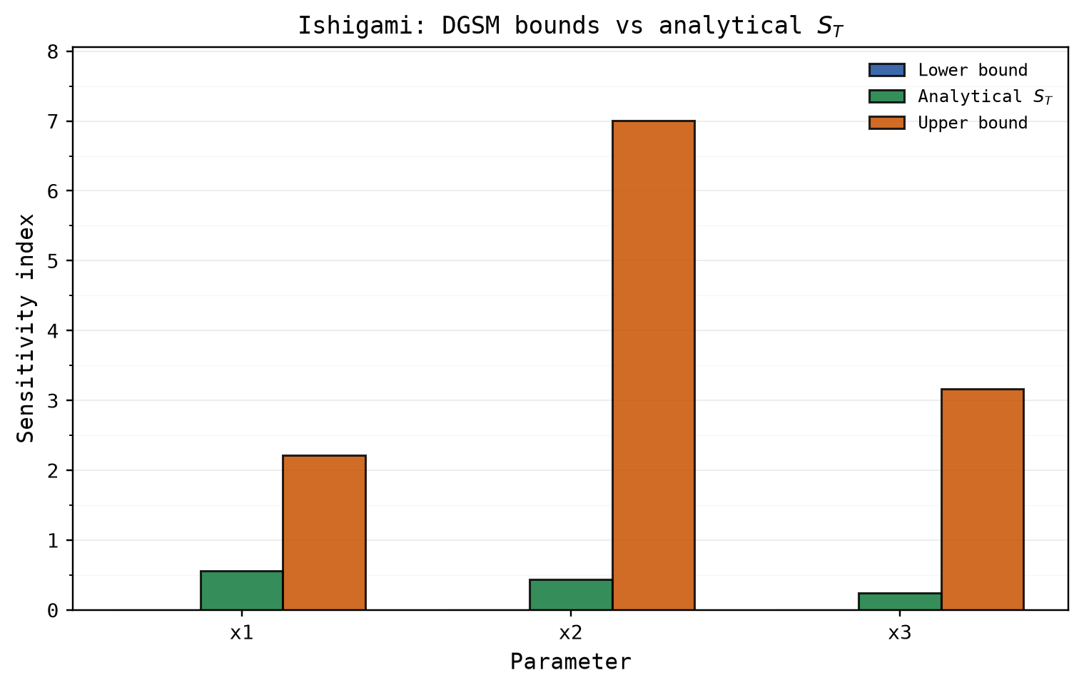
examples/dgsm_benchmark.py runs the same call against two benchmarks with closed-form answers: Ishigami, which is strongly nonlinear with a pure interaction, and a purely additive linear model. The point is not the API, which the scalar example covers, but what the bracket does on each kind of function. Both problems use uniform marginals, so the script opens with the warning the previous section explains — the lower values are estimates, not floors — and adds a second one: every upper bound here exceeds 1.

Ishigami. The unbatched helper is defined once, in the (3,) -> () shape, at the only place it is used:

def ishigami_fn(x):
    """Unbatched Ishigami: (3,) -> ()."""
    A, B = 7.0, 0.1
    return jnp.sin(x[0]) + A * jnp.sin(x[1]) ** 2 + B * x[2] ** 4 * jnp.sin(x[0])

X_ish = jaxgsa.sampling.monte_carlo(ishigami.PROBLEM, n=50_000, seed=42)
result_ish = jaxgsa.dgsm.analyze(ishigami.PROBLEM, ishigami_fn, jnp.asarray(X_ish))

The script prints the nu/sigma table and the bracket:

Param	${\nu }_i$	${\sigma }_i$	Lower	$S_T$	Upper
x1	7.7162	+0.0248	0.0001	0.5576	2.2162
x2	24.4046	+0.0034	0.0000	0.4424	7.0094
x3	11.0375	+0.0009	0.0000	0.2437	3.1702

Two readings. First, the bracket contains the analytical $S_T$ for all three parameters: 0.5576, 0.4424, and 0.2437 all sit between their lower and upper values. Second, look at x3: ${\sigma }_3=0.0009$, so the lower estimate is 0.0000, yet $S_T=0.2437$ and the upper bound is 3.1702. x3 enters only through the interaction term $B{x}_3^4\sin (x_1)$, whose derivative in $x_3$ is odd; its mean over the symmetric domain is near zero, which is exactly what $\sigma \approx 0$ reports. The interaction is not lost, though: it is what keeps ${\nu }_3=11.04$ and the upper bound at 3.17.

The script also warns that every upper bound exceeds 1, the smallest being 2.22. On this benchmark the upper bound excludes nothing by itself; the value of the run is the containment check and the $\nu$ ranking (x2 > x3 > x1).

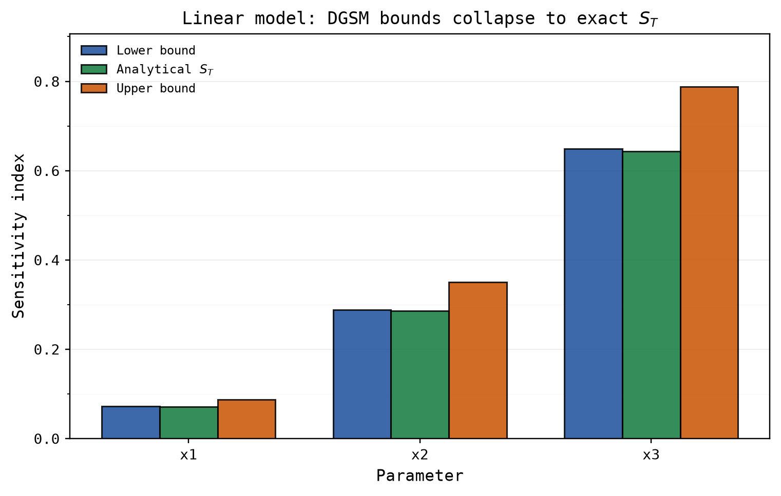
Linear model. The same pattern, with coefficients $(1,2,3)$:

def linear_fn(x):
    """Unbatched linear: (3,) -> ()."""
    c = jnp.array([1.0, 2.0, 3.0])
    return jnp.dot(c, x)

X_lin = jaxgsa.sampling.monte_carlo(linear.PROBLEM, n=10_000, seed=123)
result_lin = jaxgsa.dgsm.analyze(linear.PROBLEM, linear_fn, jnp.asarray(X_lin))

For a purely additive model the two bounds tighten onto the exact $S_T$, which for $c=(1,2,3)$ is $(1,4,9)/14$:

Param	${\nu }_i$	${\sigma }_i$	Lower	$S_T$	Upper
x1	1.0000	+1.0000	0.0720	0.0714	0.0876
x2	4.0000	+2.0000	0.2882	0.2857	0.3504
x3	9.0000	+3.0000	0.6484	0.6429	0.7883

The lower bound lands on the exact value to within Monte Carlo noise (0.6484 vs 0.6429 for x3), because for a linear response the Kucherenko-Song expression is exact. The upper bound keeps the uniform Poincare constant's slack: $12/{\pi }^2\approx 1.216$ times $S_T$, measured at 1.23 in this run. Both bounds rank the inputs exactly as $S_T$ does (x3 > x2 > x1). The full collapse of both bounds onto $S_T$ happens on Gaussian marginals, where the Poincare constant is $\mathrm{Var}(x_i)$ rather than $(b-a{)}^2/{\pi }^2$.

Forward mode or reverse mode, chosen by shape

In 1.0 there is no keyword for this. analyze counts the output slices T*K against the input count D and picks jax.jacfwd when T*K > D, otherwise jax.jacrev. The two compute the same Jacobian; only the order of the float arithmetic differs.

The choice is not cosmetic, and a time-series output is where you feel it. Reverse mode costs one pass per output, forward mode one pass per input. A model with 3 inputs and 40 output slices costs 40 reverse passes or 3 forward ones. Get that backwards on a long trajectory and the sweep is an order of magnitude slower for the same numbers.

The scalar example above printed gradients: reverse-mode autodiff (T*K=1, D=4). Give the same problem a 20-step, 2-output trajectory and the line changes:

import jax.numpy as jnp
import jaxgsa

problem = jaxgsa.Problem.from_dict(
    {"amplitude": (0.5, 2.0), "frequency": (1.0, 5.0), "damping": (0.01, 0.5)},
    output_names=("displacement", "velocity"),
)
t = jnp.linspace(0.25, 5.0, 20)


def oscillator(x):
    """Unbatched: (3,) -> (T=20, K=2)."""
    amp, freq, damping = x
    env = amp * jnp.exp(-damping * t)
    return jnp.stack(
        [env * jnp.sin(2 * jnp.pi * freq * t), env * jnp.cos(2 * jnp.pi * freq * t)],
        axis=-1,
    )


X = jaxgsa.sampling.monte_carlo(problem, n=4000, seed=0)
result = jaxgsa.dgsm.analyze(problem, oscillator, jnp.asarray(X))

print("nu shape:", result.nu.shape, "var_y shape:", result.var_y.shape)
print("damping upper_bound, displacement, t = 0.25 / 2.5 / 5.0:",
      np.round(np.asarray(result.upper_bound[[0, 9, 19], 0, 2]), 4))

jaxgsa.dgsm.analyze
  problem: D=3 (amplitude, frequency, damping)
    marginals: uniform=3
    correlation: independent
    output: N=4000 runs, T=20 x K=2 output slices
    invalid: none found in 4000 rows (policy 'raise')
  timing:
    model sweep + estimator (includes compile on the first call): 0.6434 s
    gradients: forward-mode autodiff (T*K=40, D=3)
    batch_size: auto (resolved from the memory budget)
  results: top 3 of 3 parameters by nu, mean over 40 output slices
    1. frequency  nu=82.16
    2. damping    nu=2.081
    3. amplitude  nu=0.2049
nu shape: (20, 2, 3) var_y shape: (20, 2)
damping upper_bound, displacement, t = 0.25 / 2.5 / 5.0: [0.0015 0.152  0.6083]

forward-mode autodiff (T*K=40, D=3). Forty output slices against three inputs, so forward mode wins and analyze took it without being asked. Check that line if a DGSM call is slower than you expected; it tells you which of the two counts is driving the cost, and reshaping the output is usually easier than anything else you might try.

Damping's upper bound climbs from 0.0015 to 0.61 across the trajectory. Early on you can prove damping is irrelevant. Late on you cannot prove anything, which is the correct answer, because by then it dominates. var_y has shape (T, K): one output variance per slice, and each bound is a ratio against its own slice.

Pre-computed Jacobian

If the model is not JAX-differentiable, compute the derivatives however you can and pass Y and dfdx instead of fn and X. Adjoint solvers, hand-derived formulas, and finite differences all work. dfdx mirrors Y's layout with one extra trailing (D,) axis.

import numpy as np

groundwater = jaxgsa.Problem.from_dict(
    {
        "inflow": (2.0, 8.0),
        "porosity": (0.1, 0.4),
        "roughness": (0.02, 0.05),
        "tracer": (0.0, 1.0),
    }
)

X = np.asarray(jaxgsa.sampling.monte_carlo(groundwater, n=2000, seed=0), dtype=np.float32)
q, p, k, c = X[:, 0], X[:, 1], X[:, 2], X[:, 3]

Y = q / p + 40.0 * np.sqrt(k) + 0.02 * c
dfdx = np.stack([1.0 / p, -q / p**2, 20.0 / np.sqrt(k), np.full_like(c, 0.02)], axis=-1)
print("Y:", Y.shape, "dfdx:", dfdx.shape)

precomputed = jaxgsa.dgsm.analyze(groundwater, Y=Y, dfdx=dfdx)
print("upper_bound:", precomputed.upper_bound)

Y: (2000,) dfdx: (2000, 4)
jaxgsa.dgsm.analyze
  problem: D=4 (inflow, porosity, roughness, tracer)
    marginals: uniform=4
    correlation: independent
    output: N=2000 runs, T=1 x K=1 output slice
    invalid: none found in 2000 rows (policy 'raise')
  timing:
    estimator (includes compile on the first call): 0.3863 s
    gradients: user-supplied dfdx
    batch_size: auto (resolved from the memory budget)
  results: top 4 of 4 parameters by nu
    1. porosity   nu=3.198e+04
    2. roughness  nu=1.229e+04
    3. inflow     nu=24.98
    4. tracer     nu=0.0004
upper_bound: [5.1130295e-01 1.6365178e+00 6.2900642e-03 2.2747044e-07]

The gradients: line reads user-supplied dfdx, and the bounds match the autodiff run at n=2000 to every printed digit. That is the useful check when you are unsure your hand-derived Jacobian is right. Differentiate a simplified version of the model in JAX and compare the two.

The (fn, X) group and the (Y, dfdx) group are alternatives, not a menu. Mix them and you get a ValueError naming what you passed:

ValueError: Provide either (fn, X) or (Y, dfdx), not both: got fn, X from the autodiff path and Y from the pre-computed path. Drop Y to differentiate the model, or drop fn, X to use the values you already have.

Half-filling one group raises the same way. Nothing is dropped in silence.

Note the dtype=np.float32 cast. JAX defaults to 32-bit and truncates a float64 Y on the way to the device, so the cast makes the precision you get explicit. A float64 Y is accepted too, and jaxgsa warns about it only when the values themselves do not survive float32. Turn on float64 with jax.config.update("jax_enable_x64", True) if you need it.

xarray export

This picks the result back up from the oscillator example, whose output has a time axis.

ds = result.to_dataset(time_coords=np.asarray(t))
print(ds)

<xarray.Dataset> Size: 2kB
Dimensions:      (time: 20, output: 2, param: 3)
Coordinates:
  * time         (time) float32 80B 0.25 0.5 0.75 1.0 1.25 ... 4.25 4.5 4.75 5.0
  * output       (output) <U12 96B 'displacement' 'velocity'
  * param        (param) <U9 108B 'amplitude' 'frequency' 'damping'
Data variables:
    nu           (time, output, param) float32 480B 0.4374 1.95 ... 164.8 4.129
    sigma        (time, output, param) float32 480B -0.007867 ... 0.02931
    upper_bound  (time, output, param) float32 480B 0.1278 4.051 ... 0.6083
    lower_bound  (time, output, param) float32 480B 1.487e-05 ... 0.0001041

Then ds.upper_bound.sel(param="damping", output="displacement") is the bound curve plotted above, by name instead of by index. For scalar output the dataset has a param dimension only.

Shape rules

fn signature	nu / sigma / upper / lower	var_y
(D,) -> ()	(D,)	()
(D,) -> (K,)	(K, D)	(K,)
(D,) -> (T, K)	(T, K, D)	(T, K)

D is always the last axis of the index arrays. Two output axes are the most fn may return; a third is what a batch callable produces, so analyze rejects it.

On the pre-computed path, dfdx mirrors Y with one extra trailing (D,): (N, D) for (N,) Y, (N, K, D) for (N, K), and (N, T, K, D) for (N, T, K).

Practical caveats

• The Poincare upper bound is loose for strongly nonlinear or non-monotone responses, and it can exceed 1, at which point it says nothing. It tightens towards equality as the model becomes monotone in that input. For a purely additive linear model both bounds collapse onto the exact ST.
• lower_bound is a proven floor only for a Gaussian marginal (Kucherenko & Song 2016, Theorem 6). On a uniform or truncated marginal it is exact for a linear response and can sit above the true ST for a strongly curved one, as shown above. Treat it there as an estimate, not a floor.
• Poincare constants by marginal: (b-a)^2 / pi^2 for uniform [a, b], s^2 for N(mu, s^2), and a finite-element spectral solve for a truncated normal. The truncated-normal solve is memoised per process, so repeated calls on the same marginal pay for it once.
• standardize_outputs=True divides each output slice by its own standard deviation. nu scales by a^2 and sigma by a under Y -> a*Y + b, so this is what makes slices of different magnitude comparable. The two bounds are ratios and do not move.
• on_invalid checks the derivative as well as the output, on both calling conventions. A derivative that blows up ruins nu even where the output itself is finite, and the report names "Y or its derivative" when the derivative is the culprit.
• batch_size sizes the row block on the autodiff path and bounds peak memory. None derives it from the active memory budget, pricing each row at roughly T*K*D floats. It never changes which algorithm runs.
• A var_y near zero makes both bounds a ratio of two small numbers, and analyze warns for any output slice with zero variance.
• DGSM refuses a Problem with categorical inputs: a derivative along an unordered level code has no meaning, and a categorical marginal has no Poincare constant. It also refuses a declared correlation, because both inequalities assume the inputs are independent.

See also

• Basic example for the Sobol workflow when you need the exact variance shares the bounds only bracket.
• Morris for the same screening idea with finite differences instead of derivatives, for models JAX cannot differentiate.
• eFAST for frequency-based variance decomposition.
• PCE for analytical Sobol indices from expansion coefficients.
• Methods for the theory and the method comparison.
• API reference for every parameter.