Benchmarks

These benchmarks answer two separate questions:

1. How did the performance branch change jaxgsa itself?
2. How does jaxgsa analysis time compare with SALib on the same data?

Both suites time the analysis step, not model evaluation or sampling. The results describe the workloads and machine below; they are not package limits.

Results at a glance

Across the 27-case jaxgsa workload matrix, the performance branch reduced the sum of warm median analysis times from 0.921 s to 0.430 s, a 53% reduction. The geometric mean fell from 6.98 ms to 5.14 ms. The largest isolated gains were in HSIC and VKOGA; most methods changed little because the branch did not rewrite their main estimator.

Against SALib, scalar work remains the least favourable case for JAX. The advantage grows when one call analyzes many output slices or bootstrap replicates, because jaxgsa keeps that work inside compiled array programs.

Environment

All results on this page were measured on 15 September 2026 with:

Component	Value
Machine	MacBook Pro with Apple M1 Pro, 8 CPU cores, 16 GB memory
Operating system	macOS 15.6.1, arm64
Python	3.12.13
jaxgsa	0.9.0 development tree
JAX / jaxlib	0.10.2 / 0.10.2
NumPy	2.4.2
SALib	1.5.2
Backend	JAX CPU, float32

No GPU or TPU result is inferred from these CPU measurements.

Performance branch against master

The all-method harness runs every case in a fresh subprocess. It records the first call separately, then reports the median of nine warm calls. Each call blocks until its JAX arrays are ready. Expected jaxgsa warnings and verbose reports are disabled inside the timed region.

The baseline is commit 94a4043 on master. The candidate is performance PR #80 at commit 4215d19 plus the benchmark-only suppression of reports and expected warnings. Both use the same harness, environment, seed, inputs, and process-isolation policy.

Representative warm results

Workload	Shape	master	PR	Ratio	Peak RSS: master → PR
Sobol, small	$D=3$, $N=1024$, scalar	0.86 ms	0.52 ms	1.7x	72 → 55 MiB
Sobol, high sample count	$D=3$, $N=65536$, scalar	1.96 ms	1.01 ms	1.9x	60 → 33 MiB
Sobol, high dimension with $S_2$	$D=30$, base $N=8192$, scalar	7.37 ms	3.45 ms	2.1x	108 → 66 MiB
Sobol, time series	$D=3$, $N=8192$, 300 slices	17.21 ms	9.00 ms	1.9x	202 → 96 MiB
Sobol, bootstrap	$D=3$, $N=4096$, 32 slices, 100 resamples	74.88 ms	48.85 ms	1.5x	333 → 173 MiB
Kucherenko	$D=10$, $N=8192$, 32 slices	22.21 ms	17.83 ms	1.2x	110 → 107 MiB
HSIC	$D=3$, $N=512$, scalar, 10 permutations	152.95 ms	23.10 ms	6.6x	344 → 318 MiB
VKOGA	$D=3$, $N=512$, scalar	348.29 ms	27.15 ms	12.8x	328 → 202 MiB

The 27 cases deliberately include small problems, high $N$, high $D$, multi-output/time-series arrays, and bootstrap workloads across all thirteen methods. The complete machine-readable results are available for the baseline and performance branch.

Aggregate results

Metric across 27 isolated cases	master	PR	Change
Sum of warm medians	0.921 s	0.430 s	−53%
Geometric mean of warm medians	6.98 ms	5.14 ms	−26%
Sum of per-case peak RSS deltas	3968 MiB	3304 MiB	−17%
Largest per-case peak RSS delta	344 MiB	318 MiB	−7%

The memory sum is an aggregate comparison, not simultaneous memory use: each case runs in a separate process. RSS is a process high-water mark, so small differences near the existing high-water mark are noisy.

The branch is not faster in every case. Several sub-millisecond cases sit near the dispatch and timer floor, and the 512-slice Sobol and PAWN cases varied by a few percent between runs. The large HSIC, VKOGA, and Sobol changes are well above that noise.

Comparison with SALib

The competitor benchmark runs jaxgsa and SALib on identical arrays. It reports the best of repeated warm calls, so these numbers answer a narrower question than the median-based branch comparison above.

The Sobol and HDMR benchmark first checks both libraries on the Ishigami model. All gated Sobol comparisons passed against SALib and the analytical indices. HDMR-to-analytical rows remain informational because a low-order surrogate is not exact for Ishigami.

Sobol without bootstrap

D=5, base $N=1024$. The second-order design contains 12,288 model outputs; the first/total-only design contains 7,168.

Output shape	jaxgsa, no $S_2$	SALib, no $S_2$	Ratio	jaxgsa with $S_2$	SALib with $S_2$	Ratio
1 × 1	0.6 ms	0.2 ms	0.4x	0.8 ms	0.8 ms	1.0x
1 × 6	0.6 ms	1.3 ms	2.1x	0.9 ms	5.1 ms	5.4x
50 × 1	1.1 ms	11.8 ms	10.6x	1.7 ms	43.6 ms	25.9x
50 × 6	4.4 ms	71.6 ms	16.1x	7.4 ms	262.8 ms	35.4x

Sobol with 300 bootstrap resamples

Output shape	jaxgsa, no $S_2$	SALib, no $S_2$	Ratio	jaxgsa with $S_2$	SALib with $S_2$	Ratio
1 × 1	4.1 ms	23.2 ms	5.6x	6.7 ms	69.7 ms	10.4x
1 × 6	15.7 ms	121.7 ms	7.8x	42.1 ms	397.9 ms	9.4x
50 × 1	263.6 ms	1119.6 ms	4.2x	434.2 ms	3393.5 ms	7.8x
50 × 6	1363.3 ms	7422.8 ms	5.4x	2754.9 ms	22841.6 ms	8.3x

HDMR

maxorder=2, m=2, 1,024 random samples, no bootstrap.

Output shape	jaxgsa	SALib	Ratio
1 × 1	7.0 ms	81.8 ms	11.6x
1 × 6	6.4 ms	479.0 ms	74.3x
50 × 1	10.3 ms	3629.6 ms	352.1x
50 × 6	23.8 ms	25973.1 ms	1089.7x

The largest ratios measure architecture as much as arithmetic. SALib runs one HDMR analysis per output slice in Python, while jaxgsa fits all slices in one compiled call. Quote the workload with the ratio; 1089.7x is specifically a 300-slice comparison against single-process SALib.

Four-method comparison

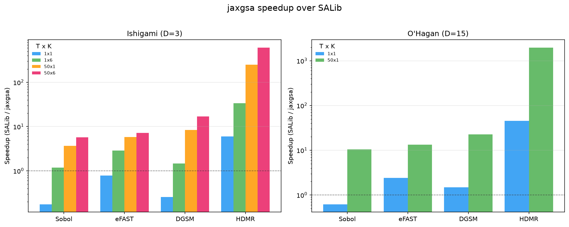
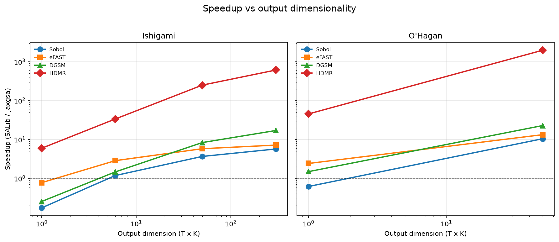
The supplemental benchmark covers Sobol, eFAST, DGSM, and HDMR on Ishigami ($D=3$) and Oakley--O'Hagan ($D=15$). These are analysis timings, not accuracy results. DGSM also differs in what is timed: jaxgsa receives a precomputed Jacobian, while SALib computes finite differences inside its analysis call.

Problem and output	Sobol	eFAST	DGSM	HDMR
Ishigami, 1 × 1	0.2x	0.8x	0.3x	6.0x
Ishigami, 50 × 6	5.7x	7.2x	17.0x	609.7x
O'Hagan, 1 × 1	0.6x	2.4x	1.5x	45.4x
O'Hagan, 50 × 1	10.4x	13.3x	22.8x	1968.1x

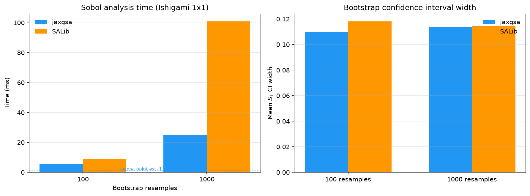
Ratios above 1 mean jaxgsa was faster. The generated figures retain every scenario:

What the benchmarks do not show

• Model evaluation and sampling are excluded. For an expensive simulator, estimator speed may have little effect on total study time.
• The SALib baseline is single-process CPU execution. No claim is made against a user-written parallel wrapper.
• First calls include tracing and compilation. The warm figures apply after compiled programs are reusable for the same shapes.
• The branch matrix uses method-specific benchmark settings; it does not rank the scientific value or accuracy of different sensitivity measures.
• Surrogate timings do not establish surrogate quality. Check the fit before interpreting PCE, HDMR, Shapley, or VKOGA indices.
• Results on other hardware and software versions will differ.

Reproduce the results

Run the all-method branch matrix:

uv run .auto/bench_gsa.py --repeats 9 --out benchmark.json

Run the correctness-checked Sobol and HDMR comparison:

uv run --extra dev benchmark_salib.py

Regenerate the four-method cache and figures:

uv run --extra dev examples/benchmark_all.py --refresh

Use an otherwise idle machine. Record the exact commit, hardware, dependency versions, backend, dtype, sample dimensions, and whether the figures are cold or warm whenever you publish new numbers.

Analytical benchmark functions

jaxgsa.benchmarks ships five models with analytical or published reference indices. Use them to test estimator accuracy separately from runtime.

Module	Parameters	Marginals	Useful check
ishigami	3	Uniform $[-\pi ,\pi ]$	Separates a zero first-order effect from a non-zero total effect
sobol_g	8	Uniform $[0,1]$	Provides clear influential and nearly inert parameter tiers
linear	3	Uniform $[0,1]$	Has equal first/total indices and zero interactions
gaussian_linear	3	Gaussian	Includes analytical Borgonovo and optimal-transport indices
oakley_ohagan	15	Gaussian	Tests a flatter, interaction-rich sensitivity profile

Each module provides a PROBLEM, batched evaluate(X), and analytical or published arrays. Read the module API for non-default parameters and the method comparison example for a worked accuracy comparison.