Benchmarks

Two separate things live on this page, and they answer different questions.

The test functions answer "is this method correct?". Their indices are known in closed form, so you can measure an estimator's error rather than guess at it.

The timing comparison answers "how long does the analysis step take against SALib on one CPU core?". Read the caveats before you quote a number from it. Every speedup on this page is measured against single-process NumPy, and the biggest ones measure a Python loop rather than arithmetic.

Test functions

jaxgsa.benchmarks ships five analytical models. Each submodule provides a PROBLEM, a batched evaluate(X), precomputed ANALYTICAL_* arrays, and an analytical_*(...) function for non-default parameters.

All five give S1, ST and S2. Three of the five also give Shapley effects: ishigami, sobol_g, and linear. gaussian_linear gives a Borgonovo delta and an optimal-transport index instead, which makes it the only ground truth in the library for a moment-independent estimator. oakley_ohagan gives neither Shapley effects nor a moment-independent ground truth; it ships the published PUBLISHED_S1 literal alongside its own closed-form S1/ST/S2.

Module	D	Marginals	Extra ground truth
ishigami	3	uniform on $[-\pi ,\pi ]$
sobol_g	8	uniform on $[0,1]$
linear	3	uniform on $[0,1]$
gaussian_linear	3	$\mathcal{N}(0,1)$	ANALYTICAL_DELTA, ANALYTICAL_OT
oakley_ohagan	15	$\mathcal{N}(0,1)$	PUBLISHED_S1

ishigami

$f(x)=\sin (x_1)+A{\sin }^2(x_2)+B{x}_3^4\sin (x_1)$, with $x_i\sim U[-\pi ,\pi ]$ and defaults $A=7$, $B=0.1$.

Pick this one when you want to check that a method separates a zero first-order effect from a non-zero total effect. $x_3$ enters only through its interaction with $x_1$, so the exact answer is $S_1=0$ and $S_T=0.2437$. A method that reports $x_3$ as unimportant has failed.

Exact	$x_1$	$x_2$	$x_3$
ANALYTICAL_S1	0.3139	0.4424	0.0000
ANALYTICAL_ST	0.5576	0.4424	0.2437
ANALYTICAL_SHAPLEY	0.4357	0.4424	0.1218

evaluate(X, A=7.0, B=0.1) maps (N, 3) to (N,). analytical_indices(A=7.0, B=0.1) returns (S1, ST, S2); analytical_shapley(A=7.0, B=0.1) returns the effects.

The $[-\pi ,\pi ]$ domain and A=7, B=0.1 are the SALib convention, and jaxgsa pins them as the default because at least three conventions circulate in the literature with very different indices (A=7, B=0.05 gives S1=0.2185; A=2, B=1 gives S1=0.3830). Other papers use other constants and get different reference numbers, so check the domain and both constants before you compare against a published table, and treat a published Ishigami table as unverified until you have re-derived at least one row. Azzini and Rosati (2022), Data in Brief 42:108071, for example, prints a first-order 0.4413 for $x_2$ against a total of 0.4424111. $x_2$ has no interactions, so the two must be equal, and it is the first-order figure that is wrong.

sobol_g

$g(\mathbf{x})=\prod _{j=1}^D\frac{|4x_j-2|+a_j}{1+a_j}$ with $x_j\sim U[0,1]$.

Eight dimensions, and the a vector sets importance directly: $a_j=0$ makes $x_j$ maximally influential, and a large $a_j$ makes it nearly inert. The default a = (0, 1, 4.5, 9, 99, 99, 99, 99) gives four tiers, with the last four parameters at $S_1\approx {10}^{-4}$.

Pick this one to test screening. A screening method has to put those four parameters at the bottom and keep them there. The exact S1 is [0.7162, 0.1790, 0.0237, 0.0072, 0.0001, 0.0001, 0.0001, 0.0001].

evaluate(X, a=DEFAULT_A) maps (N, 8) to (N,).

linear

$f(\mathbf{x})=\sum _j{c}_j{x}_j$ with $x_j\sim U[0,1]$ and $c=(1,2,3)$.

The model is purely additive, so $S_1=S_T=(0.0714,0.2857,0.6429)$ and every second-order index is exactly zero. That exact zero is the point: use it to check that a method does not manufacture interactions out of sampling noise.

analytical_indices(coeffs, bounds) covers other coefficients and other bounds.

gaussian_linear

The same additive model with $x_j\sim \mathcal{N}(0,{\sigma }_j^2)$.

Gaussian marginals make the output and every conditional output Gaussian, so more than the variance indices come out in closed form. analytical_delta computes the Borgonovo delta from a closed-form L1 distance between Gaussians plus a 1-D Gauss-Hermite quadrature (quad_order=61 by default), giving ANALYTICAL_DELTA = [0.0890, 0.2016, 0.3874]. analytical_ot gives ANALYTICAL_OT = [0.0364, 0.1548, 0.4024].

This is the only ground truth in the library for jaxgsa.borgonovo and jaxgsa.optimal_transport. Every other benchmark checks variance-based methods only.

oakley_ohagan

Oakley and O'Hagan (2004), 15 dimensions: $f(\mathbf{x})={\mathbf{a}}_1^{\mathrm{\top }}\mathbf{x}+{\mathbf{a}}_2^{\mathrm{\top }}\sin (\mathbf{x})+{\mathbf{a}}_3^{\mathrm{\top }}\cos (\mathbf{x})+{\mathbf{x}}^{\mathrm{\top }}M\mathbf{x}$ with $x_i\sim \mathcal{N}(0,{\sigma }^2)$.

The only benchmark here with more than 8 dimensions, and one of the few standard sensitivity benchmarks with Gaussian rather than uniform inputs. The inputs are independent; the quadratic form creates every pairwise interaction between their effects, and no single parameter dominates: the largest $S_1$ is 0.136 and the largest $S_T$ is 0.155. That flat profile is harder for a ranking method than Ishigami is.

The module carries PUBLISHED_S1, the reference table from the paper, next to the derivation-based ANALYTICAL_S1. They agree to 1.7e-5, which is what you would expect from a table printed to six decimals. If you change the derivation, that comparison is the test that catches you.

Measuring an estimator's error

import jaxgsa
from jaxgsa.benchmarks import ishigami

sr = jaxgsa.sobol.sample(ishigami.PROBLEM, 65536, seed=0, verbose=False)
result = jaxgsa.sobol.analyze(sr, ishigami.evaluate(sr.samples), verbose=False)

print("max S1 error:", abs(result.S1 - ishigami.ANALYTICAL_S1).max())
print("max ST error:", abs(result.ST - ishigami.ANALYTICAL_ST).max())

max S1 error: 0.00041368604
max ST error: 0.00035494566

Note that sobol.sample takes a total run count, not a base sample count. At n_samples=65536 with D=3 and second-order on, the base sample is 8192 and you evaluate 65536 rows.

Repeating that with seed=0 at three sizes gives the convergence you should expect from a Saltelli column-swap design on this function:

n_runs	max $|S_1-\text{exact}|$	max $|S_T-\text{exact}|$
8,192	0.00842	0.00239
65,536	0.00041	0.00035
524,288	0.00002	0.00000

Each 8x in n_runs cuts the error by about 20x. Plain Monte Carlo would give $\sqrt{8}\approx 2.8$x, so the scrambled Sobol' sequence is doing real work here, which is what you expect on a smooth low-dimensional function. Do not read these as tolerances for your own model. They are the error on this function, at this seed, in float32.

Timing against SALib

The comparison times the analysis step only, which computes indices from outputs you already have. Model evaluation is excluded, and on a real model that is where almost all the wall time goes. A 100x speedup on a step that took 20 ms does not make your study 100x faster.

What was measured. jaxgsa.sobol.analyze with and without second-order indices, and jaxgsa.hdmr.analyze, on a coupled damped-oscillator model with D=5 parameters and base_n=1024. Four output shapes, written T x K for T timepoints and K outputs.

Hardware and versions. Apple M1 Pro (8 cores, 6 performance and 2 efficiency), CPU only, no GPU. macOS, Python 3.12.13, JAX 0.10.2, SALib 1.5.2. Every number in the tables below was re-measured on this software stack for the 1.0 release, not carried over from an earlier one.

Method. Best of 5 identical runs on the same data, except the SALib HDMR path at best of 2 because each of its slices costs about a second. The jaxgsa figures are post-JIT steady state; the one-off XLA compile, 0.3 to 1.1 s depending on the shape, is paid once per process and excluded. SALib is pure NumPy and SciPy and needs no compilation. Every jaxgsa call runs with verbose=False, and every timed jaxgsa result is blocked with jax.block_until_ready before the clock stops.

The baseline is one CPU core

Every "speedup" below is single-process jaxgsa on an M1 Pro CPU against single-process NumPy SALib on one core of the same machine, which is what SALib does by default. It is not a comparison against a parallel CPU baseline or a tuned GPU, where published speedups for Monte Carlo GSA are closer to 13x. The large HDMR numbers in particular come from SALib running a Python loop over output slices. See what the timings do not measure.

Sobol, no bootstrap

D=5, base_n=1024, n_bootstrap=0. Speedup is SALib time divided by jaxgsa time, so above 1.0 means jaxgsa is faster.

Scenario (T x K)	Method	jaxgsa (ms)	SALib (ms)	Speedup
1 x 1	analyze, no S2	0.9	0.2	0.2x
1 x 1	analyze with S2	1.3	0.8	0.6x
1 x 6	analyze, no S2	1.3	1.4	1.0x
1 x 6	analyze with S2	1.7	5.5	3.3x
50 x 1	analyze, no S2	3.5	12.5	3.6x
50 x 1	analyze with S2	4.3	45.4	10.6x
50 x 6	analyze, no S2	13.0	74.4	5.7x
50 x 6	analyze with S2	19.1	285.6	15.0x

The two 1 x 1 rows are the honest ones. On a single scalar output SALib is faster, by about 4x without second order. There is not enough work in a D=5, N=1024 scalar analysis to pay back JAX dispatch, and no amount of kernel fusion fixes that. Use jaxgsa there for the gradients and the device placement, not for the milliseconds.

Sobol, 300 bootstrap resamples

Same design, n_bootstrap=300.

Scenario (T x K)	Method	jaxgsa (ms)	SALib (ms)	Speedup
1 x 1	analyze, no S2	31.7	20.8	0.7x
1 x 1	analyze with S2	33.9	70.3	2.1x
1 x 6	analyze, no S2	44.2	143.0	3.2x
1 x 6	analyze with S2	71.7	459.4	6.4x
50 x 1	analyze, no S2	508.1	1134.3	2.2x
50 x 1	analyze with S2	613.4	3782.6	6.2x
50 x 6	analyze, no S2	2541.4	7964.0	3.1x
50 x 6	analyze with S2	3662.6	23805.1	6.5x

Bootstrap narrows the gap rather than widening it. The resampling itself is O(n_bootstrap) work on both sides, so the fixed per-slice Python cost that jaxgsa avoids becomes a smaller share of the total. The scalar no-S2 case is still a loss.

HDMR

maxorder=2, m=2, 1,024 random samples, no bootstrap.

Scenario (T x K)	jaxgsa (ms)	SALib (ms)	Speedup
1 x 1	7.4	80.3	10.9x
1 x 6	8.2	513.1	62.9x
50 x 1	9.5	3958.9	417.2x
50 x 6	27.4	29059.7	1060.1x

Do not quote the 1060x on its own. It is 300 output slices against single-process SALib, and SALib refits its whole HDMR backfitting loop once per slice in Python. jaxgsa fits all 300 in one compiled pass, and its own time only grows from 7.4 ms to 27.4 ms across a 300-fold increase in output slices. That flatness is the real finding. The ratio is mostly a statement about how SALib is structured.

eFAST, DGSM, and the 15-D case

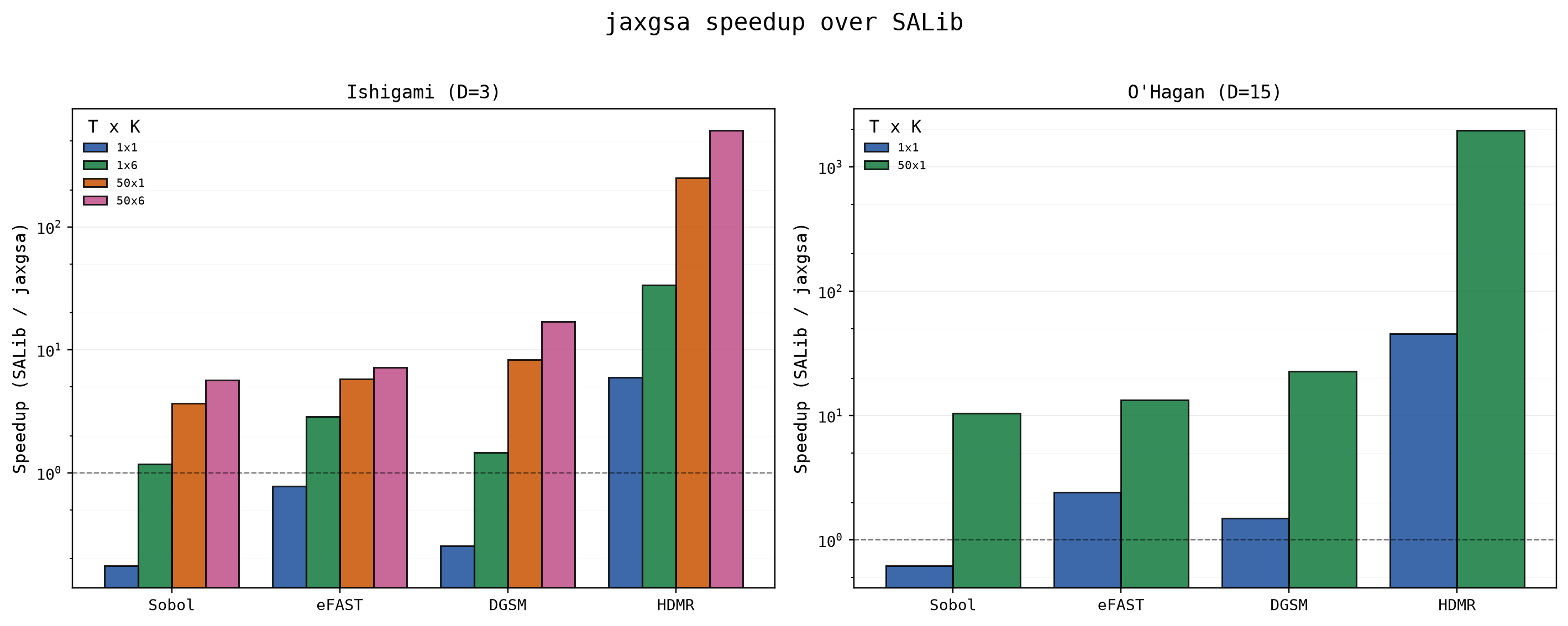
The oscillator benchmark above covers Sobol and HDMR. A second script, examples/benchmark_all.py, adds eFAST and DGSM, and runs both problems this page already uses — Ishigami (D=3) and Oakley-O'Hagan (D=15) — so the effect of dimension is visible in the same table. Same measurement rules as the oscillator benchmark: analysis step only, best of 3, verbose=False, blocked before the clock stops. The numbers below are the cache-backed run (examples/benchmark_cache.json), so they are reproducible without re-running the benchmark.

eFAST. eFAST evaluates the model along sinusoidal search curves — one per parameter — and reads $S_1$ and $S_T$ out of the Fourier spectrum of the output. Both libraries use n_per_curve=2049, M=4. jaxgsa matches or beats SALib on every row except the scalar one, which is a tie:

Problem	Scenario (T x K)	jaxgsa (ms)	SALib (ms)	Speedup
Ishigami (D=3)	1x1	0.6	0.5	1.0x
Ishigami (D=3)	1x6	1.1	2.9	2.7x
Ishigami (D=3)	50x1	5.7	24.1	4.2x
Ishigami (D=3)	50x6	23.1	155.6	6.7x
O'Hagan (D=15)	1x1	1.0	2.4	2.5x
O'Hagan (D=15)	50x1	22.7	122.8	5.4x

DGSM. The two libraries are not timing the same job. The jaxgsa row times jaxgsa.dgsm.analyze(problem, Y=..., dfdx=...) on a pre-computed Jacobian; the autodiff sweep that produces dfdx is excluded from the timer. The SALib row times SALib.analyze.dgsm.analyze(...) on finite-difference samples, and the finite differences are computed inside the timed region, so SALib pays for derivative work that the jaxgsa timer does not:

Problem	Scenario (T x K)	jaxgsa (ms)	SALib (ms)	Speedup
Ishigami (D=3)	1x1	0.6	0.3	0.4x
Ishigami (D=3)	1x6	0.4	1.5	3.6x
Ishigami (D=3)	50x1	0.9	13.1	14.7x
Ishigami (D=3)	50x6	5.4	88.3	16.3x
O'Hagan (D=15)	1x1	0.6	1.4	2.2x
O'Hagan (D=15)	50x1	1.3	68.5	53.7x

Higher D amplifies the gap. Every method's speedup grows between Ishigami (D=3) and O'Hagan (D=15). The 50x1 rows show the pattern: DGSM goes from 14.7x to 53.7x, HDMR from 84.8x to 980.2x, Sobol from 1.7x to 3.8x, and eFAST from 4.2x to 5.4x. The D=15 HDMR 50x1 row is the extreme: SALib takes 60,039.5 ms — about a minute — for 50 slices, against jaxgsa's 61.3 ms. The SALib analysis time grows far faster with dimension than jaxgsa's does: on DGSM 50x1, SALib goes from 13.1 ms to 68.5 ms while jaxgsa goes from 0.9 ms to 1.3 ms. The ratio widens because SALib re-enters Python once per output slice, and each slice's work grows with D; see where the difference comes from.

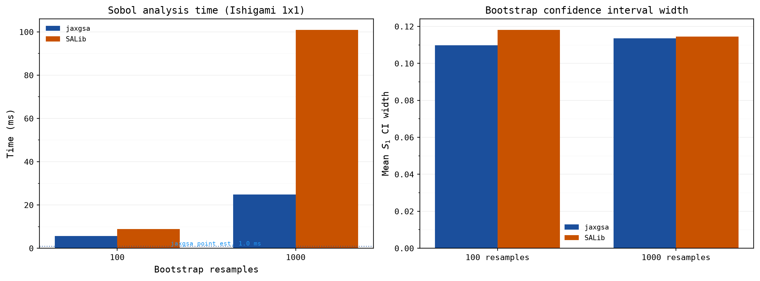
Bootstrap confidence intervals. The script also compares bootstrap confidence intervals on Ishigami 1x1 Sobol (base_n=1024, ci_method="gaussian" on both sides). The mean $S_1$ CI width lands in the same range in both libraries: jaxgsa 0.146 at 100 resamples and 0.156 at 1000; SALib 0.115 at 100 and 0.113 at 1000. jaxgsa's measured width runs about a quarter to a third wider at each count, and neither width narrows from 100 to 1000 resamples. The flatness is the expected bootstrap behavior: the resample count $B$ sets how precisely the width is estimated, and that error falls like $1/\sqrt{B}$, while the width itself is set by the base sample size. The resampling cost is where jaxgsa pulls ahead: 4.9 ms and 16.8 ms at 100 and 1000 resamples against SALib's 8.6 ms and 108.3 ms (jaxgsa's no-resample point estimate is 1.2 ms).

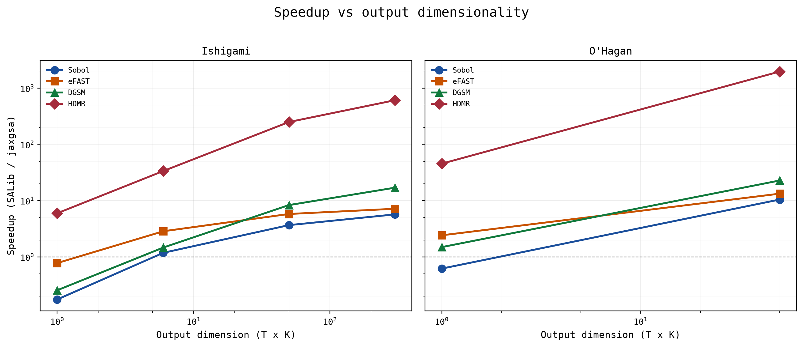
Speedup tracks T x K. The scaling story is the same one this page tells for the oscillator: the ratio grows with the output slice count, and the scalar rows remain the weak spot — Sobol 1x1 is 0.1x on Ishigami and 0.5x on O'Hagan, DGSM 1x1 is 0.4x — for the reasons given in where the difference comes from. eFAST 1x1 is a tie and HDMR 1x1 still wins (24.9x at D=15), because SALib's HDMR is heavy even for one slice.

The script. benchmark_all.py is a plain script: it runs top to bottom, prints the tables above, and shows three figures. Results cache to examples/benchmark_cache.json, and the default run loads that cache; pass --refresh to re-run the benchmarks:

uv run --extra dev python examples/benchmark_all.py

Unlike benchmark_salib.py, benchmark_all.py has no correctness gate: it does not check jaxgsa against SALib or against the analytical indices. benchmark_salib.py is the correctness-checked reproduction behind this page's Sobol and HDMR tables.

Where the difference comes from

SALib analyzes each (t, k) output slice in a Python loop. For the 50 x 6 case that is 300 sequential calls into the analyzer, each with its own array allocations and its own pass over the sample.

jaxgsa does four things differently.

• One fused kernel per call. It computes the pooled variance once and derives every S1, ST and S2 index from it, instead of recomputing it 2D times per output slice.
• jax.vmap over all T*K slices in a single compiled pass, so the per-slice Python cost disappears.
• A scalar fast path when T*K == 1, which skips the vmap machinery entirely.
• JIT, so a bootstrap loop or a parameter sweep reuses one compiled kernel while SALib re-enters Python every time.

That is why the ratio tracks T*K and not D. SALib's cost is linear in the slice count; jaxgsa's is close to flat until the arrays stop fitting in cache. At T*K == 1 the ordering flips and SALib wins, because jaxgsa still pays JAX dispatch overhead on a job too small to amortize it.

What the timings do not measure

Four limits, in the order a reviewer will raise them.

The baseline is single-process NumPy on one core. SALib does not parallelize its output-slice loop, and the benchmark does not add parallelism for it. A user with P cores can run that loop across P processes and divide the SALib column by up to P. This machine has 8 cores, so a perfectly parallel SALib would cut the HDMR 50 x 6 ratio from 1060x to about 130x. Quote the table as "against single-process SALib", never as "faster than SALib".

The largest ratios measure loop overhead, not arithmetic. The HDMR 50 x 6 number is dominated by 300 Python-level refits. It says jaxgsa's vectorization removes a scheduling cost that SALib pays. It does not say jaxgsa's floating point is hundreds of times faster, and it does not transfer to a workload with one output slice, where the same comparison gives 10.9x.

Cost claims carry a T factor. Every speed or cost statement in this project states T or says it is scalar-output-only. One reverse-mode pass returns one row of the Jacobian, so a model with T*K output slices costs T*K reverse passes. The textbook argument that a gradient costs about 3 model runs, and so beats a N*(D+2) Saltelli design for D >= 2, holds only at T*K = 1. At T*K = 10 the crossover moves to D > 28. This is why jaxgsa.dgsm picks jax.jacfwd when T*K > D and jax.jacrev otherwise. A benchmark table that does not say what T was is not comparable.

These are CPU numbers. No GPU or TPU figures appear on this page, because none have been measured on hardware this project controls. Published speedups for large Monte Carlo GSA on a GPU against a fully parallel CPU sit near 13x, so treat a GPU as a further win of about that size at most, not as a multiplier on the tables above.

Setup and reproduction

• Model: coupled damped oscillators, D=5 parameters, T timepoints, K outputs.
• Samples: base_n=1024 Sobol' points. That is 7,168 evaluated rows for first and total order, and 12,288 with second order.
• Bootstrap: 300 resamples for the bootstrap tables, 0 for the others.
• HDMR: maxorder=2, m=2, on the same 1,024 random samples.
• Correctness: before it times anything, the script checks jaxgsa against SALib on identical Ishigami data (D=3, n_runs=131072) and checks jaxgsa Sobol against the analytical solution. The HDMR-versus-analytical rows are printed for context and do not gate the pass, because RS-HDMR at maxorder=2 does not converge to the exact indices on Ishigami.

The script is benchmark_salib.py in the repository root. SALib is a dev extra, so the run needs --extra dev:

uv run --extra dev python benchmark_salib.py

It prints the correctness table first, then the timing tables. Your numbers will differ with hardware, and the T*K == 1 rows are close enough that they can change sign between machines.

Figures

The companion script also draws three figures: